Limits to Arbitrage and Investor Anomalies
Investment Theory
Fall 2026
Why Doesn’t Arbitrage Fix Prices?
- The efficient markets argument has two steps:
- Irrational investors push prices away from fundamental values.
- Rational arbitrageurs trade against them, push prices back, and take their money.
- If some anomalies are mispricing, the second step must fail somewhere.
- This chapter:
- Why arbitrage may not correct prices.
- Cases where mispricing is beyond doubt.
- How individual investors actually behave.
What Arbitrage Requires
- Real-world “arbitrage”: buy what looks cheap, sell a close substitute that looks expensive, and wait.
- Barberis and Thaler (2003): this can be risky and costly even when the mispricing is large.
- Fundamental risk: substitutes are rarely perfect.
- Noise trader risk: the mispricing can get worse before it gets better.
- Implementation costs: commissions, spreads, price impact, and above all shorting costs.
- “Prices are right” implies “no free lunch”, but not the reverse.
- Pontiff (2006): idiosyncratic risk keeps positions small, \propto \alpha / \sigma^{2}(e), as in Treynor-Black.
Noise Trader Risk
- De Long et al. (1990): an asset with no fundamental risk, worth 1, and a fraction \mu of noise traders who misperceive its future price by \rho_{t} \sim N(\rho^{*}, \sigma_{\rho}^{2}).
- The price is p_{t} = 1 + \frac{\mu (\rho_{t} - \rho^{*})}{1 + r} + \frac{\mu \rho^{*}}{r} - \frac{2 \gamma \mu^{2} \sigma_{\rho}^{2}}{r (1 + r)^{2}}.
- The last term: sophisticated investors fear noise traders will be even more pessimistic when they sell, and require a premium.
- Noise traders “create their own space”.
- Noise traders with moderate optimism can earn higher expected returns, though with lower expected utility.
Performance-Based Arbitrage
- Shleifer and Vishny (1997): arbitrageurs manage other people’s money, and investors judge them by their returns.
- Noise traders depress the price by S_{t}; arbitrageurs invest D_{1} out of funds F_{1}, so p_{1} = V - S_{1} + D_{1}.
- After losses, investors withdraw money: F_{2} = F_{1} - a D_{1} \left( 1 - \frac{p_{2}}{p_{1}} \right) \qquad p_{2} = V - S_{2} + F_{2}. \tag{1}
- With a > 1, arbitrageurs are forced to sell when the mispricing is largest.
Example 1 (Arbitrageurs Forced to Sell) Let V = 1, F_{1} = 0.2, S_{1} = 0.3 and a = 1.2, so D_{1} = 0.2 and p_{1} = 0.9. Pessimism deepens to S_{2} = 0.4. Then F_{2} = 0.2 - 1.2 \times 0.2 \times (1 - p_{2} / 0.9) and p_{2} = 0.6 + F_{2}, which give p_{2} = 0.7636 and F_{2} = 0.1636. If capital did not respond to returns, the price would be 0.8.
A Longer Episode
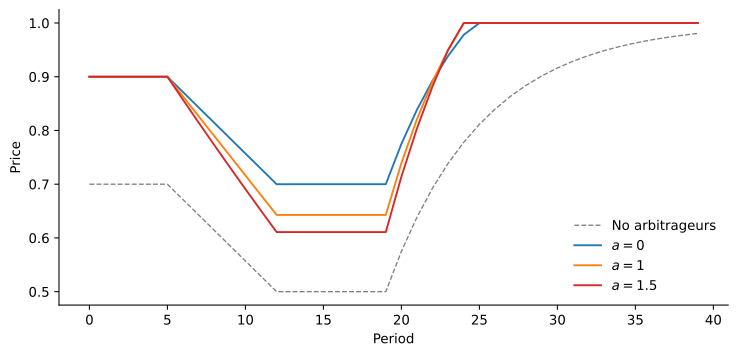
Price of a stock worth 1 when noise trader pessimism rises from 0.3 to 0.5 and then fades, with arbitrage capital that responds to returns with sensitivity a. The dashed line is the price without arbitrageurs.
- The price falls to 0.70 with a = 0, 0.64 with a = 1 and 0.61 with a = 1.5.
Arbitrage in Practice
- Shleifer and Vishny’s predictions:
- Arbitrage concentrates where trades can be hedged and converge quickly: bonds and currencies.
- Mispricing is largest where idiosyncratic volatility is high.
- Long-Term Capital Management, 1998: convergence trades moved against it during the Russian crisis, its capital shrank, and its lenders took it over.
Riding Bubbles
- Abreu and Brunnermeier (2003): arbitrageurs learn of an overpricing one by one, not knowing how many others know.
- Selling too early forgoes gains, so they ride the bubble for a while.
- Brunnermeier and Nagel (2004): hedge funds in the technology bubble.
- By March 2000, tech was 31% of their stock portfolios against 21% of the market.
- They sold individual stocks before their peaks, earning abnormal returns.
- Tiger shunned tech, lost a quarter of its assets to withdrawals, and closed in March 2000.
- Quantum raised its tech share from under 20% to about 60% in 1999, then lost heavily.
- Being right is not enough: timing matters.
Short-Sale Constraints
- Miller (1977): if investors disagree and few can sell short, the most optimistic hold the stock and set its price.
- More disagreement means a higher price relative to the average valuation.
- Short-sale constraints make overpricing more common than underpricing.
- D’Avolio (2002), 2000 to 2001:
- 91% of stocks cost less than 1% a year to borrow, most about 0.15%.
- 9% are “special”, averaging 4.3%; Krispy Kreme reached 50%, Palm 35%.
- Special stocks are small, held by few institutions, and the subject of disagreement.
Example 2 (Optimists Set the Price) Ten investors value a stock at $20, $22, and so on up to $38, each buys one share if the price is at or below their valuation, and three shares are available. The price is the third-highest valuation, $34, against an average of $29. If valuations spread to $11, $15, and so on up to $47, the average is still $29, but the price rises to $39.
Twin Shares: Royal Dutch and Shell
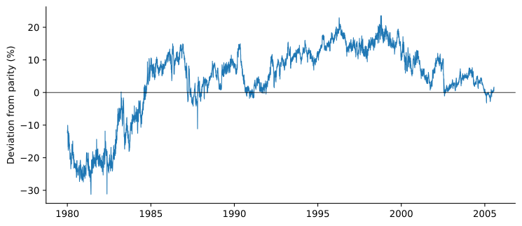
Deviation of the relative price of Royal Dutch and Shell Transport from 60:40 parity, in percent, from their U.S. listings. The parity level is set at the 2004-2005 unification.
- Royal Dutch was entitled to 60% of the group’s cash flows and Shell to 40%, so Royal Dutch should be worth 1.5 times Shell.
Mispricing without a Deadline
- Royal Dutch was 31% below parity in June 1981 and 24% above in October 1998.
- Froot and Dabora (1999): the relative price moved with the markets where each stock mainly traded.
- Location of trade affected prices, though cash flows were fixed by contract.
- The trade has no fundamental risk but no convergence date: pure noise trader risk.
- An arbitrageur who bought Royal Dutch 10% below parity in March 1983 saw it fall further for six months.
Carve-Outs: 3Com and Palm
- March 2, 2000: 3Com sold 5% of Palm in an IPO and planned to give its shareholders about 1.525 Palm shares per 3Com share.
- A 3Com share was worth at least 1.525 Palm shares. Its other value is the stub: \text{stub} = P_{\text{3Com}} - 1.525 \, P_{\text{Palm}}.
- First day: Palm $95.06, 3Com $81.81, so the stub was -$63.16.
- The market valued 3Com’s other businesses at about -\$22 billion.
The Stub over Time
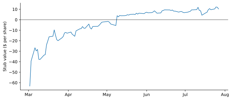
Stub value of 3Com, in dollars per share, from Palm’s IPO on March 2, 2000, to the distribution in late July 2000.
- Short interest in Palm reached 147.6% of its shares; borrowing was scarce and expensive.
- Lamont and Thaler (2003): “not an exploitable arbitrage opportunity” but “a case of blatant mispricing”.
Example 3 (A Negative Stub) A parent trades at $70 and will distribute 1.5 shares of a subsidiary trading at $50; it also holds $8 a share in cash. The stub is 70 - 75 = -\$5, though it should be at least $8. Buying the parent and shorting 1.5 subsidiary shares brings in $5, and the parent’s remaining business is worth at least $8. But borrowing the subsidiary for four months at 40% a year costs 0.40 \times 4/12 \times 75 = \$10, leaving $3.
Where Arbitrage Is Costly
- Mitchell et al. (2002): 82 negative stubs, 1985 to 2000.
- In 30% the link broke before convergence; the median time to convergence was 92 days.
- Baker and Wurgler (2006): after high sentiment, small, young, unprofitable, volatile and non-dividend-paying stocks earn low returns.
- Stambaugh et al. (2012): eleven anomalies are stronger after high sentiment, almost entirely in the short leg.
- Overpricing needs short sales to correct; underpricing does not.
Anomalies after Publication
- McLean and Pontiff (2016), 97 predictors: returns are 26% lower after the sample ends and 58% lower after publication.
- The 26% bounds statistical bias; the extra 32% is the effect of publication.
- The decline is larger where arbitrage is cheaper.
- Trading volume and short interest in the predictor portfolios rose after publication.
Publication in the JKP Factors
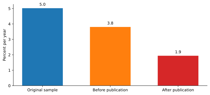
Average annual return of the JKP factors significant in the original sample, in three periods.
- 77 of 142 factors were significant in their original samples.
- Their returns fall 24% after the sample and 61% after publication, but do not disappear.
Investor Anomalies
- Limits to arbitrage explain why mispricing survives, not where it comes from.
- We need investors whose demand does not follow fundamental value, and whose errors are shared.
- Evidence from the trading records of individual investors, and from experiments.
- Barberis and Thaler (2003): overconfidence, reading too much into small samples, anchoring, and preferences that depart from expected utility.
Prospect Theory
- Kahneman and Tversky (1979):
- 82% prefer 2,400 for sure to (2,500, 0.33; 2,400, 0.66; 0, 0.01).
- 83% prefer (2,500, 0.33) to (2,400, 0.34), the same choice with a 0.66 chance of 2,400 removed.
- People prefer a 0.80 chance of losing 4,000 to a sure loss of 3,000.
- The theory:
- Gains and losses relative to a reference point, not final wealth.
- Concave for gains, convex for losses.
- Steeper for losses: “losses loom larger than gains”.
- Small probabilities are overweighted.
The Disposition Effect
- Investors who measure gains and losses from the purchase price should sell winners too early and hold losers too long.
- Odean (1998), 10,000 brokerage accounts, 1987 to 1993:
\begin{aligned}
\text{PGR} & = \frac{\text{realized gains}}{\text{realized gains} + \text{paper gains}}, \\
\text{PLR} & = \frac{\text{realized losses}}{\text{realized losses} + \text{paper losses}}.
\end{aligned}
- PGR = 0.148 and PLR = 0.098: a winner is about 50% more likely to be sold.
- Taxes favor the opposite; only in December do investors realize losses at a higher rate.
- Winners sold beat losers kept by 3.4 percentage points over the next year.
Overconfidence and Attention
- Overconfidence (Barber and Odean 2000, 2001):
- The most active households earned 11.4% a year net, against 17.9% for the market.
- Men traded 45% more than women, which cost them 2.65 points a year against 1.72.
- Attention (Barber and Odean 2008; Barber et al. 2022):
- Individuals buy stocks in the news, with high volume or extreme returns.
- Stocks Robinhood users herded into had abnormal returns of about -4.7\% over the next 20 days.
Diversification Mistakes
- Home bias (French and Poterba 1991): investors held 93.8% (U.S.), 98.1% (Japan) and 82% (U.K.) of their stock portfolios at home.
- Mean-variance reasoning would require them to expect several points a year more from domestic stocks.
- Naive diversification (Benartzi and Thaler 2001): people split money evenly across the options offered.
- Stocks get 54%, 73% or 35% depending on the menu of funds, not on attitudes to risk.
Lottery Stocks and Extrapolation
- Kumar (2009): low-priced stocks with high idiosyncratic volatility and skewness.
- Individuals hold them at about three times their market weight; the investors resemble state lottery buyers.
- Their four-factor alpha is about 7% a year lower than other stocks’.
- Greenwood and Shleifer (2014): six surveys of expected stock returns, 1963 to 2011.
- Investors expect high returns after the market has risen.
- Their expectations are negatively correlated with model-based expected returns.
- These patterns matter for prices only if they are shared and arbitrage is limited.
Takeaways
- Arbitrage is risky and costly: noise trader risk, capital that flees after losses, short-sale constraints and idiosyncratic risk.
- Twin shares and carve-outs show mispricing beyond doubt, and how hard it is to correct.
- Mispricing is largest where arbitrage is hardest, and anomalies shrink once arbitrageurs learn of them.
- Investors’ systematic patterns, from the disposition effect to extrapolation, supply the demand that arbitrage fails to offset.