Utility Theory Under Uncertainty
Investment Theory
Fall 2026
Introduction
- In a single period model, agents must decide today how much to consume and how much to save for later.
- In this presentation we take that decision as given, and assume that agents derive their utility from consumption at the end of the period.
- As is common in finance, consumption is represented by a single good.
- Agents prefer more to less, but the marginal utility of each additional unit of consumption is decreasing, i.e., the last bite is never as good as the first one.
Utility Functions
- A utility function is a function u: \mathbb{R}^{+} \rightarrow \mathbb{R}.
- The domain of the utility function is real consumption and therefore cannot be negative.
- In the following, we assume that u(c) is continuous and differentiable of all orders.
- The level of utility is not important, and can even be negative, but we assume that the utility function is increasing and strictly concave.
- In some cases it will also be useful to consider utility functions such that u'(0) = \infty, that is, in starvation an extra unit of consumption provides an infinite amount of extra utility.
Common Utility Functions
- A common choice of utility function is u(c) = \dfrac{c^{1 - \gamma} - 1}{1 - \gamma}, \text{ where $\gamma > 0$.}
- A special case occurs when \gamma = 1, since \lim_{\gamma \rightarrow 1} \frac{c^{1 - \gamma} - 1}{1 - \gamma} = \lim_{\gamma \rightarrow 1} \frac{1 + (1 - \gamma) \ln(c) - 1}{1 - \gamma} = \ln(c).
- This function is called power utility if \gamma \neq 1 and log utility if \gamma = 1.
- Another common utility function is u(c) = - e^{-a c}, called the exponential utility function.
Expected Utility and Risk Aversion
- Denote by W the wealth of the agent at the end of the period.
- This wealth is generated by investing a certain amount today.
- In general, W is unknown today and can be thought as a random variable defined over a probability space (\Omega, \operatorname{P}).
- The utility derived by a random consumption \overset{\sim}{W} is given by U(\overset{\sim}{W}) = \operatorname{E}(u(\overset{\sim}{W})).
Risk Aversion
- Consider now a random variable \tilde{\varepsilon} such that \operatorname{E}(\tilde{\varepsilon}) = 0 and \operatorname{V}(\tilde{\varepsilon}) > 0.
- We say that an agent is risk-averse if she prefers a certain level of wealth W over a random payoff with the same expected value.
- If we define \overset{\sim}{W} = W + \tilde{\varepsilon}, we have that \operatorname{E}(\overset{\sim}{W}) = W,\,\operatorname{V}(\overset{\sim}{W}) > 0 = \operatorname{V}(W).
- Thus, the agent is risk-averse if u(W) > \operatorname{E}(u(W + \tilde{\varepsilon})).
Why Concavity Means Risk Aversion
- A gamble pays W - \Delta or W + \Delta with equal probability, so \operatorname{E}(\overset{\sim}{W}) = W.
- Expected utility is the height of the chord at W, which concavity places below the curve.
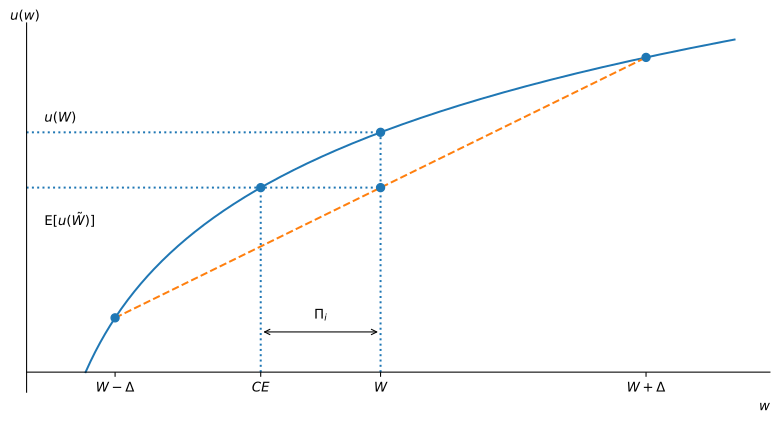
Figure 1: A concave utility function, Jensen’s inequality, and the insurance premium.
Jensen’s Inequality
- Let f: D \rightarrow \mathbb{R} be a twice-continuously differentiable and strictly concave function, and X a random variable defined in a probability space (\Omega, \operatorname{P}) such that the range of X is contained in the domain of f, and \operatorname{V}(X) > 0.
- Then we have that f(\operatorname{E}(X)) > \operatorname{E}(f(X)).
- Jensen’s inequality shows that strict concavity in u implies risk-aversion.
- The converse is also true (see notes)
- An agent is risk averse if and only if her utility function is strictly concave.
The Insurance Premium
- In many situations, we are forced to take on a risky gamble.
- For example, if you buy a car you face the risk of an accident and costly repairs.
- Many people choose to pay for insurance and hence reduce the risk of the car.
- Consider: u(W - \Pi_{i}) = \operatorname{E}(u(W + \tilde{\varepsilon})).
- The value of \Pi_{i} that solves the equation is called the insurance premium.
The Certainty Equivalent
- The agent is indifferent between the risky gamble and the certain wealth W - \Pi_{i}, which we call the certainty equivalent: CE = W - \Pi_{i}.
- Premiums rank risk aversion only across agents facing the same gamble at the same wealth: the one willing to pay more for insurance is more risk averse.
- For a single agent, \Pi_{i} varies with W, so her premiums at different wealth levels say nothing about a change in her risk aversion.
Example 1 Suppose the economy can be in one of the following two states: (i) Boom or “good” state and (ii) Recession or “bad” state, which can occur with equal probability. Consider a risky asset that would have a price of $50 in the good state and $10 in the bad state, which currently trades at $30. Two investors are evaluating this asset.
The utility function of the first investor (A) is u(W) = 10 \ln(W), whereas for the second investor (B) we have u(W) = 2W + 5.
What is the maximum price that investors A and B would be willing to pay for the risky asset?
Solution
- The expected utility of the risky asset for investor A is E(U) = 0.5 (10 \ln(10)) + 0.5(10 \ln(50)) = 31.0730.
- Therefore, \begin{aligned} 10 \ln(CE) & =31.0730 \\ CE & = \exp(3.1073) = \$22.36. \end{aligned}
- For investor B, the expected utility of the risky asset is E(U) = 0.5 (2 \times 10 + 5) + 0.5 (2 \times 50 + 5) = 65, so that \begin{aligned} 2 \times CE + 5 & = 65 \\ CE & = \$30. \end{aligned}
Example 2 Suppose that your utility function is given by \ln(W).
Assuming an initial wealth of $1,000, what is the maximum price would you be willing to pay for a lottery ticket which offers the possibility to win $5,000 with a 1% probability and nothing with a 99% probability? \ln(1000) = 0.01 \ln(1000 - P + 5000) + 0.99 \ln(1000 - P). This equation, though, can only be solved numerically. Using a solver we find P = 17.90.
Does your answer changes if your initial wealth is $10,000? \ln(10000) = 0.01 \ln(10000 - P + 5000) + 0.99 \ln(10000 - P), which yields P = 40.60.
Example 3 You have a logarithmic utility function u(W) = \ln(W), and your current level of wealth is $10,000.
Imagine you are in a situation where there’s a 50/50 chance of either winning or losing $1,500. What is the maximum amount of insurance that you are willing to pay to avoid completely the risk?
We solve \ln(CE) = 0.5 \ln(10{,}000 + 1{,}500) + 0.5 \ln(10{,}000 - 1{,}500), which gives CE = \exp(0.5 \ln(10{,}000 + 1{,}500) + 0.5 \ln(10{,}000 - 1{,}500)) = \$9{,}886.86. The insurance premium is then equal to 10{,}000 - 9886.86 = \$113.14.
Example 4 (Choosing an Insurance Plan) An investor with u(W) = \ln W and wealth $10,000 faces a 10% chance of a loss that reduces wealth to $1,000. Plan A pays $5,000 after a loss and costs $500; Plan B pays $8,000 and costs $800. Both are actuarially fair, so every choice leaves expected wealth at $9,100. The certainty equivalents are CE_{\text{none}} = \$7{,}943, \qquad CE_{A} = \$8{,}994, \qquad CE_{B} = \$9{,}095. Plan B wins: it shrinks the gap between good- and bad-state wealth the most, from $9,000 with no insurance to $4,000 under A and $1,000 under B.
Local Risk Aversion
- Intuitively, a function that is more concave should induce more risk aversion than a function that is less concave.
- We can formalize this intuition by looking at the insurance premium for a gamble with a very small variance.
- Let \operatorname{E}(\tilde{\varepsilon}) = 0 and \operatorname{V}(\tilde{\varepsilon}) > 0.
- We know that the insurance premium \Pi_{i} solves u(W - \Pi_{i}) = \operatorname{E}(u(W + \tilde{\varepsilon})).
- We can approximate the insurance premium as: \Pi_{i} \approx -\frac{1}{2} \frac{u''(W)}{u'(W)} \sigma_{\varepsilon}^{2}.
Derivation
- First, do a Taylor expansion of first order of u(W - \Pi_{i}) around W: \begin{aligned} u(W - \Pi_{i}) & \approx u(W) + u'(W) (W - \Pi_{i} - W) \\ & = u(W) - u'(W) \Pi_{i}. \end{aligned}
- Second, do a Taylor expansion of second order of u(W + \tilde{\varepsilon}) around W: \begin{aligned} u(W + \tilde{\varepsilon}) & \approx u(W) + u'(W) (W + \tilde{\varepsilon} - W) + \frac{1}{2} u''(W) (W + \tilde{\varepsilon} - W)^{2} \\ & = u(W) + u'(W) \tilde{\varepsilon} + \frac{1}{2} u''(W) \tilde{\varepsilon}^{2} \\ \operatorname{E}(u(W + \tilde{\varepsilon})) & \approx u(W) + \frac{1}{2} u''(W) \sigma^{2}_{\varepsilon}. \end{aligned}
Absolute and Relative Risk Aversion
- We denote by \mathit{ARA} = - \frac{u''(W)}{u'(W)} the coefficient of absolute risk-aversion, and by \mathit{RRA} = - \frac{u''(W)}{u'(W)} W the coefficient of relative risk-aversion.
Example
- Take u(W) = \frac{W^{1 - \gamma} - 1}{1 - \gamma}
- Then u'(W) = W^{-\gamma} and u''(W) = -\gamma W^{-\gamma - 1}, implying that \mathit{RRA} = -\left( \frac{-\gamma W^{-\gamma -1}}{W^{-\gamma}}\right) W = \gamma
- Power utility is an example of a function that exhibits constant relative risk-aversion.
Example 5 (Exponential Utility) For u(W) = -e^{-aW} with a > 0, we have u'(W) = a e^{-aW} and u''(W) = -a^{2} e^{-aW}, so \mathit{ARA} = \frac{a^{2} e^{-aW}}{a e^{-aW}} = a. Exponential utility exhibits constant absolute risk-aversion (CARA): the dollar premium \Pi_{i} \approx \frac{1}{2} a \sigma_{\varepsilon}^{2} does not depend on wealth.
How Risk Aversion Changes with Wealth
- Power utility has \mathit{ARA} = \gamma / W, which falls as wealth grows: decreasing absolute risk-aversion (DARA).
- Exponential utility keeps \mathit{ARA} = a at every wealth level.
- Most evidence and introspection favor DARA: wealthier people pay less in dollars to avoid the same gamble.
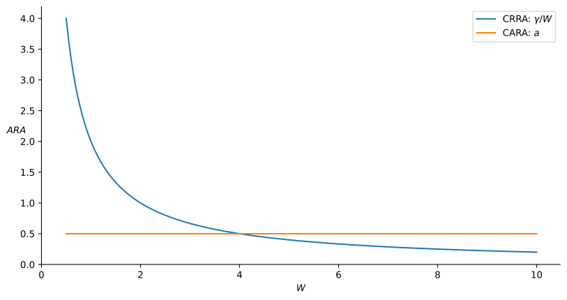
Figure 2: Absolute risk-aversion for CRRA (power) versus CARA (exponential) utility.
Proportional Gambles
- For a gamble proportional to wealth, \tilde{\varepsilon} = W \tilde{\delta} with \operatorname{E}(\tilde{\delta}) = 0 and \operatorname{V}(\tilde{\delta}) = \sigma_{\delta}^{2}, \Pi_{i} \approx \frac{1}{2} \mathit{ARA} \cdot W^{2} \sigma_{\delta}^{2} = \frac{1}{2} \mathit{RRA} \cdot W \sigma_{\delta}^{2}.
- The fraction of wealth given up is \Pi_{i} / W \approx \frac{1}{2} \mathit{RRA} \cdot \sigma_{\delta}^{2}.
- An agent with constant relative risk-aversion (CRRA), such as power utility, keeps the same fraction of wealth in risky assets however wealthy she is.
The Risk Premium
- The insurance premium asks how much an agent pays to shed a gamble she bears.
- The compensatory risk premium \Pi_{c} asks how much she must be paid to accept one: u(W) = \operatorname{E}\big(u(W + \Pi_{c} + \tilde{\varepsilon})\big). \tag{1}
- The two generally differ, since they price risk from opposite sides.
- The insurance premium is natural for casualty insurance.
- The compensatory premium is natural in finance: it is the extra expected return needed to hold a risky asset instead of a riskless one.
Two Premiums, One Curvature
- For a small gamble, the same Taylor argument gives \Pi_{c} \approx \frac{1}{2} \mathit{ARA} \cdot \operatorname{V}(\tilde{\varepsilon}), the same approximation as for \Pi_{i}.
- Both premiums are governed by the local curvature of u at W.
- In Example 1, investor A values the asset at $22.36 against an expected payoff of $30, an insurance premium of \Pi_{i} = \$7.64; the risk-neutral investor B has \Pi_{i} = \$0.