Optimal Capital Allocation
Investment Theory
Fall 2026
Introduction
The Problem
- If passive investors possess the same information, they should agree on which combination of risky assets provides the best trade off between risk and return.
- Some investors may think this optimal portfolio of risky assets carries too much risk.
- Others may think the opposite.
- It is possible to reduce or increase the risk of a portfolio by investing or borrowing a risk-free asset.
- The capital allocation decision is then about how much to invest in this well-diversified portfolio of risky investments and how much to allocate to a risk-free asset.
The Solution
- The solution to the capital allocation problem has two dimensions:
- Model what is available to invest.
- Understand what investors want.
- The first point requires us to determine the investment opportunity set.
- Combining a risky asset with the risk-free rate generates an investment set called the capital allocation line (CAL).
- The second point has to do with how investors feel when taking risks.
- Investors dislike risk but like returns.
- In finance and economics, we capture these two opposite effects using a utility function.
The Capital Allocation Line
The Economic Setup
- We analyze the investment opportunity set generated by a risky asset Q and a risk-free asset.
- We denote by r_{f} the risk-free rate of return.
- The expected return of the risky asset is denoted by \mu_{Q} whereas the standard deviation or volatility of its returns is denoted by \sigma_{Q}.
The Investment Opportunity Set
- A portfolio P that invests w in Q and 1 - w in the risk-free asset has the following expected return and volatility: \begin{aligned} \mu_{P} & = (1 - w) r_{f} + w \mu_{Q}, \\ \sigma_{P} & = |w| \sigma_{Q}. \\ \end{aligned} \tag{1}
- If we only consider portfolios in which we invest in the risky asset, i.e. w \geq 0, we can combine both equations to get \mu_{P} = r_{f} + \left( \frac{\mu_{Q} - r_{f}}{\sigma_{Q}} \right) \sigma_{P}.
The Sharpe Ratio
- The Sharpe ratio of the risky-asset is defined as: \mathit{SR} = \frac{\mu_{Q} - r_{f}}{\sigma_{Q}}. \tag{2}
- The expected return of any portfolio formed by combining the risk-free and the risky asset is given by a line with intercept r_{f} and slope coefficient \mathit{SR}: \mu = r_{f} + \mathit{SR} \times \sigma. \tag{3}
- This line is called the Capital Allocation Line of Q or just CAL(Q).
The Capital Allocation Line
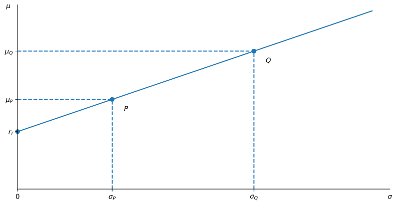
Figure 1: The figure shows the capital allocation line of the risky portfolio Q.
The CAL as a Production Function
- The CAL transforms risk into expected returns.
- The CAL of a risky asset can then be seen as a production function where the input is risk and the output is expected return.
- The Sharpe ratio of a risky asset is the marginal rate of transformation (MRT) of risk into expected return.
- Investors should then try to maximize this trade-off by maximizing the Sharpe ratio of their portfolios.
Example 1 Suppose that r_{f} = 5\%, \mu_{Q} = 12\% and \sigma_{Q} = 20\%. The Sharpe ratio of Q is \mathit{SR} = \frac{0.12 - 0.05}{0.20} = 0.35.
Suppose that you want a portfolio P on the CAL(Q) but with 5% volatility. If w denotes the weight in Q, this means that 0.05 = w \times 0.20, or w = 25\%. Thus, a portfolio that invests 25% in Q and 75% in the risk-free asset has 5% volatility. The expected return of this portfolio is: \mu_{P} = 0.75 \times 0.05 + 0.25 \times 0.12 = 6.75\%. The position of P in the CAL(Q) is illustrated in Figure 1.
Example 2 (The Capital Market Line in Practice) Highland Capital Advisors (HCA) forecasts \mu_{M} = 12\%, \sigma_{M} = 20\%, and r_{f} = 5\%. Its client Elena Cross wants a portfolio with half the volatility of the market. When the risky asset is the market portfolio, the CAL is the capital market line (CML), with slope \mathit{SR} = 0.35 as in Example 1. Cross’s constraint is \sigma_{P} = 0.5 \times 20\% = 10\%, so \mu_{P} = 0.05 + 0.35 \times 0.10 = 8.5\%. The portfolio holds w = \sigma_{P}/\sigma_{M} = 50\% in the market and 50\% in the risk-free asset.
Investor’s Utility
Expected Utility
- Investors seek to get the maximum return for the minimum risk.
- A standard way in economics to capture this trade-off is by using a utility function.
- A utility function allows us to rank different combinations of risk and expected return.
- A simple way to do this in finance is to define: U(\mu, \sigma) = \mu - \frac{1}{2} A \sigma^{2}.
- This is the local approximation \mu - \frac{1}{2}\mathit{RRA} \cdot \sigma^{2} to the certainty-equivalent return of a proportional gamble, promoted to a utility function over any (\mu, \sigma) pair.
- With exponential utility and normal returns it holds exactly, with A equal to relative risk aversion at initial wealth.
- The coefficient A denotes how sensitive is a particular investor to risk measured here by \sigma^{2}.
- We call A the coefficient of risk-aversion.
- It is common in applications to use values for A between 1 and 4.
Indifference Curves
- There are several pairs (\mu, \sigma) that provide the same utility, i.e. for a given U and \sigma, we can always find a \mu such that: \mu = U + \frac{1}{2} A \sigma^{2}.
- These functions are called indifference curves since an investor with risk-aversion coefficient A is indifferent among any of these combinations of \mu and \sigma.
- Let’s fix A = 3 and U to be either 2%, 6% or 10%. We can now plot the corresponding indifference curves.
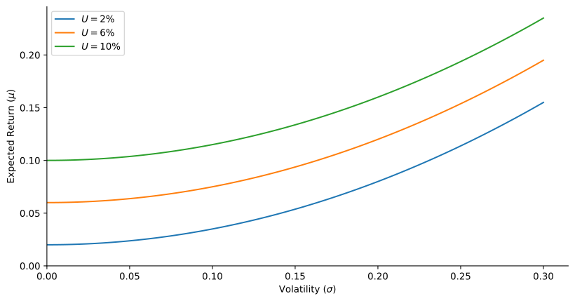
Figure 2: The figure shows indifference curves for different levels of utility.
Certainty Equivalent
- The curves in the graph represent all combinations of (\mu, \sigma) that provide the same utility, i.e. the investor is indifferent among these choices of risk and return.
- Indifference curves that provide higher utility are always above indifference curves that provide lower utility.
- Each indifference curve can be characterized by its certainty equivalent, which represents the expected return that would provide the same level of utility with no risk, that is when \sigma = 0.
- The utility level can therefore be interpreted as the certainty equivalent of a particular portfolio.
Maximizing Utility
The Investment Opportunity Set
- Optimal portfolio choice is about maximizing utility given the constraints imposed by the investment opportunity set.
- Remember that for a given w that determines the weight in the risk asset Q, the investment opportunity set is characterized by: \begin{align*} \mu & = (1 - w) r_{f} + w \mu_{Q}, \\ \sigma^{2} & = w^{2} \sigma_{Q}^{2}. \end{align*}
The Optimal Portfolio
- The utility of investing w in Q and the rest in the risk-free asset: \begin{align*} U & = \mu - \frac{1}{2} A \sigma^{2} \\ & = (1 - w) r_{f} + w \mu_{Q} - \frac{1}{2} A w^{2} \sigma_{Q}^{2}. \end{align*}
- The first-order condition (FOC) is: \frac{dU}{dw} = (\mu_{Q} - r_{f}) - A w \sigma_{Q}^{2} = 0.
- The optimal w^{*} is given by: w^{*} = \frac{\mu_{Q} - r_{f}}{A \sigma_{Q}^{2}}.
The Characteristics of the Optimal Portfolio
- The amount allocated to the risky asset is smaller if the risk aversion or if its variance are larger.
- The investor’s risk aversion and the variance of the asset play the same role and are indistinguishable.
- The amount allocated to the risky asset increases with its expected return, but decreases with the risk-free rate.
- The resulting expected return and standard deviation of the optimal portfolio are given by: \begin{align*} \mu^{*} & = (1 - w^{*}) r_{f} + w^{*} \mu_{Q}, \\ \sigma^{*} & = w^{*} \sigma_{Q}. \end{align*}
Example 3 Consider an agent with a risk-aversion coefficient equal to 3. If r_{f} = 5\%, \mu_{Q} = 12\% and \sigma_{Q} = 20\% as in Example 1, we have that w^{*} = \frac{0.12 - 0.05}{3 \times 0.20^{2}} = 58.33\%. Therefore, the portfolio that maximizes the utility for the investor consists of investing 41.67% in the risk-free asset and 58.33\% in the risky asset. The expected return and volatility of this portfolio are \begin{aligned} \mu^{*} & = (1 - w^{*}) \times 0.05 + w^{*} \times 0.12 = 9.08\%, \\ \sigma^{*} & = w^{*} \times 0.20 = 11.67\%. \end{aligned}
The Optimality Condition
- The investor wants to maximize utility, i.e., to achieve the highest level of utility possible.
- The point where the indifference curve is tangent to the CAL(Q) determines the optimal portfolio.
- At this point, the marginal rate of substitution (MRS) between risk and return equals the marginal rate of transformation (MRT) between risk and return.
- This is the same tangency condition as in the Fisher model, now applied to risk and return instead of C_{0} and C_{1}.
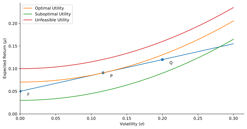
Figure 3: The figure shows that optimal portfolio choice occurs where the marginal rate of substitution equals the marginal rate of transformation between risk and return.
Computing the MRS
- The MRS characterizes the trade-off between risk and return for the same level of utility.
- In an indifference curve, we must have that 0 = dU = \frac{\partial U}{\partial \mu} d\mu + \frac{\partial U}{\partial \sigma} d\sigma = d\mu - A \sigma d\sigma. Thus, \text{MRS} = \frac{d\mu}{d\sigma} = A \sigma.
Computing the MRT
- In our setup, the MRT characterizes the ability to transform risk into expected return.
- The MRT is therefore equal to the Sharpe ratio of any portfolio on the CAL(Q), i.e. \text{MRT} = \frac{\mu - r_{f}}{\sigma}.
Finding the Optimum Again
- The optimal portfolio with mean \mu^{*} and standard deviation \sigma^{*} satisfies \text{MRS} = A \sigma^{*} = \frac{\mu^{*} - r_{f}}{\sigma^{*}} = \text{MRT}.
- We could have used this equation to find the optimal portfolio weights.
- Just replace \mu^{*} = r_{f} + w (\mu_{Q} - r_{f}) and \sigma^{*} = w \sigma_{Q} in the expression above, and solve for w.
Is There Another Way?
- Yes, we could try maximizing utility subject to the constraint of the capital allocation line given by (3), i.e., forming a Lagrangian: \mathcal{L} = \mu - \frac{1}{2} A \sigma^{2} - \lambda (\mu - r_{f} - \mathit{SR} \sigma).
- The FOC are \begin{aligned} \frac{\partial \mathcal{L}}{\partial \mu} & = 1 - \lambda = 0, \\ \frac{\partial \mathcal{L}}{\partial \sigma} & = -A \sigma + \lambda \mathit{SR} = 0,\\ \frac{\partial \mathcal{L}}{\partial \lambda} & = \mu - r_{f} - \mathit{SR} \sigma = 0. \\ \end{aligned}
- The solution is the same as before, i.e., \text{MRS} = \text{MRT}.