The Greeks

Options, Futures and Derivative Securities

Lorenzo Naranjo

Spring 2026

From Replication to Hedging

From Replication to Hedging

• Black-Scholes prices an option by replication: holding N_{S} = \partial V / \partial S shares and rebalancing continuously reproduces the option exactly.
• A desk that sells an option can hold the same portfolio as a hedge: the position is then delta neutral.
  • A static hedge with other options is sometimes available, but often not feasible or too expensive.
• In practice the desk rebalances at discrete times, once a day or once a week, and between trades the hedge is imperfect.
• The other Greeks measure what goes wrong between trades and what else the position is exposed to.

Delta

Delta of a Portfolio

• The delta of an option (or portfolio) measures its sensitivity to the underlying asset price: \Delta = \frac{\partial V}{\partial S}
• The delta of a portfolio is the sum of the deltas of its positions.
  • A share has a delta of one and a bond a delta of zero, so the desk adjusts delta by trading the stock.
• The delta of a European call or put is the Black-Scholes hedge ratio.

Example 1

• Consider a non-dividend paying stock that currently trades at $50.
• The money-market risk-free rate is 5% per year with continuous compounding, and the volatility of log-returns is 25% per year.
• To compute the delta of a European call option with maturity 6 months and strike of $50, we first calculate d_{1} = \frac{\ln(50/50) + (0.05 + \frac{1}{2}(0.25)^{2})(0.5)}{0.25\sqrt{0.5}} = 0.2298
• The delta is then equal to \operatorname{Φ}(d_{1}) = 0.591.

Example 2: Weekly Hedge

• A trader just sold 50 call option contracts (5,000 options) on the stock of the previous example.
• The option price is $4.13 and its delta is 0.591. The money-market rate is 5% per year with simple compounding.
• First hedge: the delta of the position is -5{,}000 \times 0.591 = -2{,}955.
  • The trader buys 2,955 shares for $147,750 and receives 5{,}000 \times 4.13 = \$20{,}650 for the calls.
  • The net expense of $127,100 is borrowed at the risk-free rate.

Example 2: One Week Later

• The stock price increases to $50.53, the option price to $4.35, and the delta to 0.612.
• The stock is worth 2{,}955 \times 50.53 = \$149{,}316.15 and the short calls -5{,}000 \times 4.35 = -\$21{,}750.
• The loan accrues to -127{,}100 \left(1 + \frac{0.05}{52}\right) = -\$127{,}222.21.
• The weekly P&L is 149{,}316.15 - 21{,}750 - 127{,}222.21 = \$343.94.
  • A perfect hedge would earn nothing, so this is a hedging error. We explain it once we have gamma and theta.
• Rebalancing: the trader buys 3{,}060 - 2{,}955 = 105 shares for 105 \times 50.53 = \$5{,}305.65, borrowed, so the loan is now $132,527.86.

Example 3

• Consider:
  • A long position in 100,000 call options (1,000 contracts) with strike price $100 and expiration in 9 months. The delta of each option is 0.597.
  • A short position in 200,000 call options (2,000 contracts) with strike $110 and expiration in 6 months. The delta of each option is 0.368.
  • A short position in 50,000 put options (500 contracts) with strike $90 and expiration in 3 months. The delta of each option is -0.162.
• The delta of the portfolio is: 100{,}000 \times 0.597 - 200{,}000 \times 0.368 - 50{,}000 \times (-0.162) = -5{,}800
• The portfolio can then be made delta neutral by buying 5,800 shares.

Gamma

Gamma of a Portfolio

• The gamma (\Gamma) of a portfolio measures the rate of change of its delta with respect to the price of the underlying asset: \Gamma = \frac{\partial \Delta}{\partial S} = \frac{\partial^{2} V}{\partial S^{2}}
• Gamma is the reason a delta hedge must be rebalanced.
  • Small gamma: delta changes slowly and the hedge needs few adjustments.
  • Large gamma: the hedge must be monitored and adjusted frequently.
• For European call and put options: \Gamma_{C} = \Gamma_{P} = \frac{e^{-\delta T} \mathop{\Phi^{'}}(d_{1})}{S \sigma \sqrt{T}} = \frac{K e^{-r T} \mathop{\Phi^{'}}(d_{2})}{S^{2} \sigma \sqrt{T}}

Example 4

• The gamma of the option in Example 1, with d_{1} = 0.2298: \mathop{\Phi^{'}}(d_{1}) = \frac{1}{\sqrt{2 \pi}} e^{-\frac{1}{2} (0.2298)^{2}} = 0.3885 \Gamma = \frac{\mathop{\Phi^{'}}(d_{1})}{S \sigma \sqrt{T}} = \frac{0.3885}{50 (0.25) \sqrt{0.5}} = 0.0440

Gamma and Delta Neutrality

• According to Itô’s lemma: dV = \Delta dS + \frac{1}{2} \Gamma (dS)^{2} + \frac{\partial V}{\partial t} dt
• In a delta-neutral portfolio the first term vanishes, and over a short interval \Delta V \approx \frac{1}{2} \Gamma (\Delta S)^{2} + \frac{\partial V}{\partial t} \Delta t
• A delta-neutral portfolio is not riskless: its value moves with the square of the stock price change, and the sign of gamma decides whether large moves help or hurt.
• The stock and the bond have zero gamma, so gamma can only be changed by trading options.

Gamma and the Delta Hedge

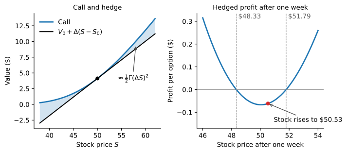
Left: the call of Example 1 and the hedge line tangent at S_0 = 50 with slope \Delta = 0.591; the shaded gap is the value of the delta-hedged long call. Right: the profit per option of the hedged long call after one week. The dashed lines mark the breakeven prices.

• Over a week the call also loses time value: the hedged long call gains only if the stock ends below $48.33 or above $51.79.
• In Example 2 the stock rose to $50.53, inside that range, so the desk, short the calls, made money.

Example 5

• Suppose that the gamma of a delta-neutral portfolio is 10,000.
• A jump of +$2 or -$2 in the underlying asset will approximately increase the value of the portfolio by \frac{1}{2} 10{,}000 \times 2^{2} = \$20{,}000.

Example 6

• A trader’s portfolio is delta-neutral and has a gamma of 5,000.
• The delta and gamma of a traded call option are 0.52 and 1.60, respectively.
• The trader wants to make the portfolio both delta and gamma-neutral.
  • The portfolio can be made gamma-neutral by selling \frac{5{,}000}{1.60} = 3{,}125 call options.
  • The portfolio can now be made delta-neutral by buying 0.52 \times 3{,}125 = 1{,}625 shares of the underlying asset.
  • The shares have zero gamma, so they do not change the gamma of the portfolio but only its delta.

Theta

Theta of a Portfolio

• The theta (\Theta) of a portfolio captures the rate of change of its value with the passage of time, its time decay: \Theta = \frac{\partial V}{\partial t}
• For European call and put options: \begin{aligned} \Theta_{C} & = - e^{-\delta T} \frac{S \mathop{\Phi^{'}}(d_{1}) \sigma}{2 \sqrt{T}} - r K e^{-r T} \operatorname{Φ}(d_{2}) + \delta S e^{-\delta T} \operatorname{Φ}(d_{1}) \\ \Theta_{P} & = - e^{-\delta T} \frac{S \mathop{\Phi^{'}}(d_{1}) \sigma}{2 \sqrt{T}} + r K e^{-r T} \operatorname{Φ}(-d_{2}) - \delta S e^{-\delta T} \operatorname{Φ}(-d_{1}) \end{aligned}

Theta and Gamma

• The Black-Scholes equation, written with the Greeks: (r - \delta) S \Delta + \frac{1}{2} \sigma^{2} S^{2} \Gamma + \Theta = r V
• For a delta-neutral portfolio: \frac{1}{2} \sigma^{2} S^{2} \Gamma + \Theta = r V
• When theta is large and positive, gamma tends to be large and negative, and vice-versa.
• In a delta-neutral book, theta is the price paid, or earned, for gamma.

The Profit of a Delta Hedge

• Long an option, short \Delta shares, with V - \Delta S financed at the risk-free rate.
• Using Itô’s lemma and the Black-Scholes equation, the profit over a short interval \Delta t is \frac{1}{2} \Gamma S^{2} \left[ \left(\frac{\Delta S}{S}\right)^{2} - \sigma^{2} \Delta t \right]
• The bracket compares the squared return the stock delivered with the variance \sigma^{2} \Delta t in the price.
  • Long gamma: gains when the stock moves more than its volatility implies, loses its theta when it moves less.
  • Short gamma, like the desk that sold calls: earns theta in quiet markets, loses when the stock moves a lot.

Example 7

• In Example 2 the desk is short 5,000 calls with S = 50, \sigma = 0.25, and \Gamma = 0.0440 per option.
• The stock rose from $50 to $50.53 in one week, so \left(\frac{\Delta S}{S}\right)^{2} = 0.000112 \quad \text{and} \quad \sigma^{2} \Delta t = \frac{0.25^{2}}{52} = 0.001202
• The stock moved less than its volatility implies, so the short calls gain about 5{,}000 \times \frac{1}{2} (0.0440) (50)^{2} \times (0.001202 - 0.000112) = \$299.75
• Most of the $343.94 of the week; the rest comes from applying an instantaneous formula to a whole week.

Hedging Over the Life of the Option

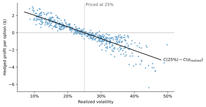
Profit per option of a short call hedged weekly at \sigma = 25\%, against the volatility realized on each of 500 simulated paths. The solid line is C(25\%) - C(\sigma_{\mathit{realized}}).

Hedging in Practice

• Desks run this calculation every day: the P&L attribution, or P&L explain, splits the day’s profit into delta, gamma, theta, and vega parts plus an unexplained residual.
• Delta-hedged long calls on the S&P 500 lost money from 1988 to 1995, about 8% of the option value at the money (Bakshi and Kapadia 2003).
  • A negative volatility risk premium: volatility rises when the market falls, so options hedge market declines and investors pay to hold them.
  • A desk that sells options and delta hedges collects that premium, as compensation for its losses in crashes.

Implied vs. Realized Volatility

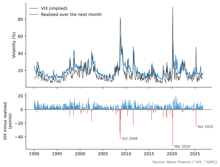
VIX at each month-end and the S&P 500 volatility realized over the following 21 trading days (top), and their difference (bottom). Source: Yahoo Finance.

• From 1990 to September 2026, the VIX exceeded the volatility that followed in 84% of months, by 4.1 points on average.

Transaction Costs

• Rebalancing more often shrinks the gamma error, but every trade costs money.
• With Black-Scholes deltas, the hedging error after costs does not shrink as rebalancing becomes more frequent (Leland 1985).
• Hedge instead with Black-Scholes at a modified variance: \hat{\sigma}^{2} = \sigma^{2} \left(1 + \sqrt{\frac{2}{\pi}} \frac{k}{\sigma \sqrt{\Delta t}}\right) where k is the round-trip cost and \Delta t the time between rebalancings.
  • Replicating the option costs more, and costs turn the Black-Scholes price into a band.

How Often to Rebalance

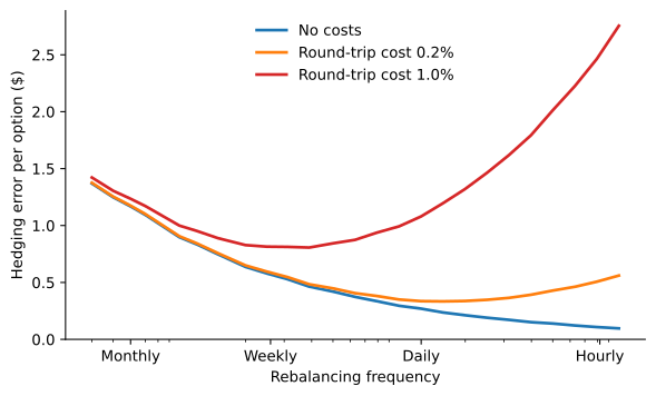
Root mean squared present value of the profit per option of a short call delta hedged with Black-Scholes deltas, against the number of rebalancings, on 4,000 paths with \sigma = 25\%. Each trade pays half the round-trip cost on the amount traded.

• Without costs, rebalancing four times as often halves the error. With costs, the best frequency falls from about daily (0.2%) to about weekly (1%).

Deep Hedging

• A neural network learns the hedge from simulated market paths (Buehler et al. 2019).
• It chooses trades to minimize a risk measure of the hedged profit after transaction costs and trading limits.
• It can hedge with liquid options as well as with the stock.
• Without costs it recovers the model hedge; with costs it trades off hedging error against trading costs.
• Risk limits and P&L reports are still expressed in Greeks, so learned hedges complement them.

Vega

Vega of a Portfolio

• Vega, met in Black-Scholes, is the sensitivity of the option to volatility, computed in practice with respect to implied volatility: \mathcal{V} = \frac{\partial V}{\partial \sigma}
• For European call and put options: \mathcal{V}_{C} = \mathcal{V}_{P} = S e^{-\delta T} \mathop{\Phi^{'}}(d_{1}) \sqrt{T} = K e^{-r T} \mathop{\Phi^{'}}(d_{2}) \sqrt{T}
• Vega risk matters most for long maturities, gamma risk for short ones.
• The stock and the bond have zero vega, so vega can only be hedged with options, and hedging gamma and vega together takes two options.

Example 8

• Consider a portfolio that is delta neutral, with a gamma of -5,000 and a vega of -8,000. The options shown in the table below can be traded.

	Delta	Gamma	Vega
Portfolio	0	-5,000	-8,000
Option 1	0.6	0.5	2.0
Option 2	0.5	0.8	1.2

• The portfolio can be made vega neutral with a long position in 4,000 units of Option 1.
• This would increase delta to 2,400, so 2,400 units of the asset must be sold to keep delta neutrality.
• The gamma of the portfolio would change from -5,000 to -3,000.

Example 8 (Continued)

• To make the portfolio both gamma and vega neutral, both Option 1 and Option 2 can be used.
• We must then solve: \begin{aligned} -5{,}000 + 0.5 N_{1} + 0.8 N_{2} = 0 \\ -8{,}000 + 2.0 N_{1} + 1.2 N_{2} = 0 \end{aligned}
• This yields N_{1} = 400 and N_{2} = 6{,}000.
  • The new delta is 400 \times 0.6 + 6{,}000 \times 0.5 = 3{,}240.
• Hence, we sell 3,240 units of the underlying asset to maintain delta-neutrality.

Dealers and Demand

• Even a delta, gamma, and vega neutral book is not riskless: dealers trade at discrete times, volatility changes, and prices jump.
• Because of this unhedgeable risk, option prices depend on demand (Garleanu et al. 2009).
  • End users are net long S&P 500 index options, especially out-of-the-money puts, so dealers are net short.
  • Demand pressure helps explain why index options are expensive and the volatility skew.
• Dealers set these prices through quotes that lean against their inventory vega (Baldacci et al. 2021).
• On exchanges, quoting is automated and dominated by high-frequency trading firms: in 2025 Morgan Stanley, the last major bank in the business, closed its automated options market-making unit and sold it to Citadel Securities (Lee and Goyder 2025; Doherty 2025).

Rho

Rho of a Portfolio

• The rho (\rho) of a portfolio measures the rate of change of its value with respect to the risk-free rate: \rho = \frac{\partial V}{\partial r}
• For European call and put options: \begin{aligned} \rho_{C} & = K T e^{-r T} \operatorname{Φ}(d_{2}) > 0 \\ \rho_{P} & = - K T e^{-r T} \operatorname{Φ}(-d_{2}) < 0 \end{aligned}
• A call is a levered position in the stock financed by borrowing: a higher rate lowers the present value of the debt.
• A put is a short position in the stock combined with lending: a higher rate lowers the present value of the loan.

Summary

Summary

• In the Black-Scholes model where dS = (r - \delta) S dt + \sigma S dB^{*}:

Variable	Call	Put
V	S e^{-\delta T} \operatorname{Φ}(d_{1}) - K e^{-r T} \operatorname{Φ}(d_{2})	K e^{-r T} \operatorname{Φ}(-d_{2}) - S e^{-\delta T} \operatorname{Φ}(-d_{1})
\Delta	e^{-\delta T} \operatorname{Φ}(d_{1})	-e^{-\delta T} \operatorname{Φ}(-d_{1})
\Gamma	\dfrac{e^{-\delta T} \mathop{\Phi^{'}}(d_{1})}{S \sigma \sqrt{T}} = \dfrac{K e^{-r T} \mathop{\Phi^{'}}(d_{2})}{S^{2} \sigma \sqrt{T}}
\Theta	r V - (r - \delta) S \Delta - \frac{1}{2} \sigma^{2} S^{2} \Gamma
\mathcal{V}	S e^{-\delta T} \mathop{\Phi^{'}}(d_{1}) \sqrt{T} = K e^{-r T} \mathop{\Phi^{'}}(d_{2}) \sqrt{T}
\rho	K T e^{-r T} \operatorname{Φ}(d_{2})	- K T e^{-r T} \operatorname{Φ}(-d_{2})

Quoting the Greeks

• Desks quote the Greeks in units that match the moves they care about:
  • Theta per calendar day, \Theta/365, or per trading day, \Theta/252.
  • Vega per volatility point, \mathcal{V}/100.
  • Delta in dollars, \Delta S.
  • Gamma as the profit from a 1% move, \frac{1}{2} \Gamma S^{2} (0.01)^{2}.

The Greeks Across Maturities

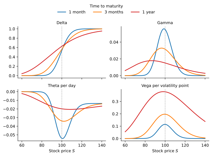
Delta, gamma, theta per day, and vega per volatility point of a call with K = 100, r = 5\%, and \sigma = 25\%.

Gamma Near Expiration

• Gamma and theta concentrate at the strike as expiration approaches; vega grows with maturity.
• Near expiration, a desk hedging an option at the strike must trade large amounts of stock whenever the price crosses it: pin risk.
• The area under gamma is always one, since delta rises from 0 to 1.
  • As maturity shrinks, that unit area piles up at the strike: gamma converges to a Dirac delta at K, the second derivative of \max(S - K, 0).

References

Bakshi, Gurdip, and Nikunj Kapadia. 2003. “Delta-Hedged Gains and the Negative Market Volatility Risk Premium.” Review of Financial Studies 16 (2): 527–66.

Baldacci, Bastien, Philippe Bergault, and Olivier Guéant. 2021. “Algorithmic Market Making for Options.” Quantitative Finance 21 (1): 85–97. https://doi.org/10.1080/14697688.2020.1766099.

Buehler, Hans, Lukas Gonon, Josef Teichmann, and Ben Wood. 2019. “Deep Hedging.” Quantitative Finance 19 (8): 1271–91. https://doi.org/10.1080/14697688.2019.1571683.

Doherty, Katherine. 2025. Citadel Securities Buys Morgan Stanley’s Options Market Maker. Bloomberg, July 10, 2025. https://www.bloomberg.com/news/articles/2025-07-10/citadel-securities-buys-morgan-stanley-s-options-market-maker.

Garleanu, Nicolae, Lasse Heje Pedersen, and Allen M. Poteshman. 2009. “Demand-Based Option Pricing.” Review of Financial Studies 22 (10): 4259–99.

Lee, Justina, and Bernard Goyder. 2025. Morgan Stanley to Shutter Electronic Equity Market-Making Unit. Bloomberg, June 18, 2025. https://www.bloomberg.com/news/articles/2025-06-18/morgan-stanley-to-shutter-electronic-equity-market-making-unit.

Leland, Hayne E. 1985. “Option Pricing and Replication with Transactions Costs.” Journal of Finance 40 (5): 1283–301.