Properties of European Options
Options, Futures and Derivative Securities
Lorenzo Naranjo
Spring 2026
The Put-Call Parity
Building a Covered Call
- Consider European call and put options with strike K and maturity T written on a non-dividend paying stock.
- There is also a zero-coupon risk-free bond with face value K and same maturity as the options.
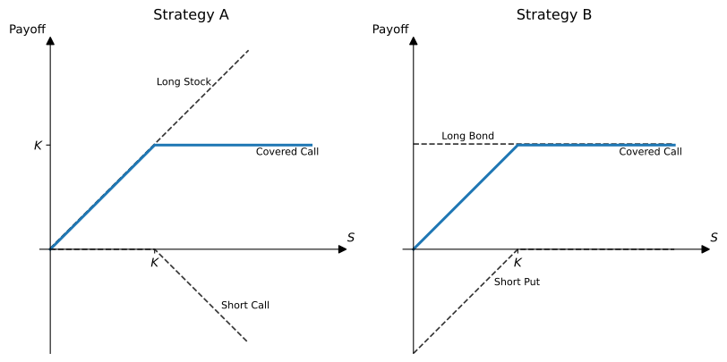
Strategy A
Long stock and short call
\begin{aligned}
\text{Cost} & = S - C \\
\text{Payoff} & =
\begin{cases}
S_{T} & \text{if $S_{T} \leq K$} \\
K & \text{if $S_{T} > K$}
\end{cases}
\end{aligned}
Strategy B
Long bond and short put
\begin{aligned}
\text{Cost} & = K e^{-r T} - P \\
\text{Payoff} & =
\begin{cases}
S_{T} & \text{if $S_{T} \leq K$} \\
K & \text{if $S_{T} > K$}
\end{cases}
\end{aligned}
Payoff Diagrams for Both Strategies
Put-Call Parity
- Since both strategies have the same payoff, they should have the same price.
- Otherwise, buy the cheapest strategy and sell the most expensive one.
- This would generate a free positive cash flow with zero risk.
- For European options written on non-dividend paying stocks, the following relationship known as put-call parity must hold: S - C = K e^{-r T} - P
Example 1
- Consider a non-dividend paying stock trading at $110 and assume that the continuously-compounded risk-free rate is 5% per year.
- A European call option with strike price $110 and maturity 9 months trades for $13.30.
- Then, according to put-call parity, we should have that a European put with the same strike and maturity as the call should cost: \begin{aligned} P & = C - S + K e^{-r T} \\ & = 13.30 - 110 + 110 e^{-0.05 \times 0.75} \\ & = 9.25 \end{aligned}
Example 2
- What if in the previous example everything stays the same, but you find that the put trades for $9?
- Then we have an arbitrage opportunity!
- Let us consider both strategies discussed previously that we know have the same payoff.
- Strategy A: Long stock and short call \text{Cost}_{A} = 110 - 13.30 = 96.70
- Strategy B: Long bond and short put \text{Cost}_{B} = 110 e^{-0.05 \times 0.75} - 9 = 96.95
- Since \text{Cost}_{A} < \text{Cost}_{B}, we should buy A and sell B which generates an instant profit of $0.25 per share.
Example 2 (cont’d)
| Position | Today | S_{T} \leq 110 | S_{T} > 110 |
|---|---|---|---|
| Long Stock | -110.00 | S_{T} | S_{T} |
| Short Call | 13.30 | 0 | 110 - S_{T} |
| Short Bond | 105.95 | -110 | -110 |
| Long Put | -9.00 | 110 - S_{T} | 0 |
| Total | 0.25 | 0 | 0 |
Put-Call Parity and Protective Puts
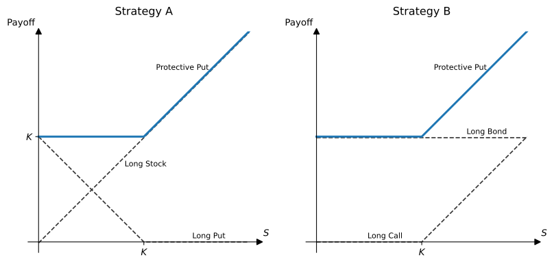
- We can also express put-call parity in the following way: S + P = K e^{-r T} + C
- The left hand-side of this expression is the cost of a protective put, i.e. long stock and long put.
- The right hand-side says that a protective put can also be built by buying a bond and a call.
Payoff Diagrams for Protective Put
Put-Call Parity and Forward Contracts
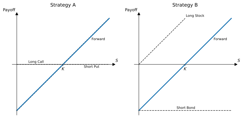
- We can express put-call parity in yet a different way: C - P = S - K e^{-r T}
- The right hand-side of this expression is the cost of a forward contract with forward price K.
- The left hand-side says that a forward contract can be synthesized by buying a call and selling a put.
Payoff Diagrams for Forward Contract
Option Pricing Bounds
A Simple Lower Bound on Call and Put Options
- The price of a European call or put option cannot be negative.
- If not, any trader would like to get as many contracts as possible.
- The worst-case scenario is that the options expire out-of-the-money in which case the payoff is zero.
- Otherwise the options expire in-the-money and the option trader gets a positive payoff.
- This would clearly be a nice arbitrage opportunity!
- Hence, we must have that C \geq 0 and P \geq 0.
Lower Bound on European Call Options
- Remember that we are analyzing an underlying asset that does not pay dividends.
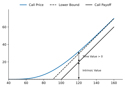
- Put-call parity and the fact that P \geq 0 implies that: C = P + S - K e^{-r T} \geq S - K e^{-r T}
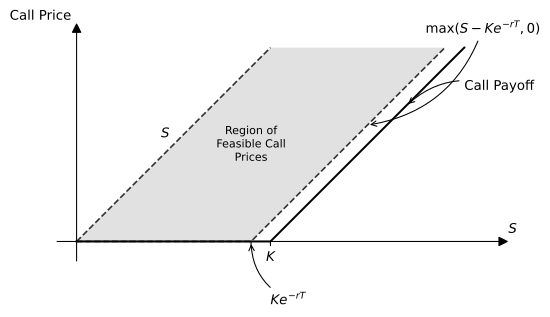
- Given that we also have C \geq 0, it must be the case that: C \geq \max(S - K e^{-r T}, 0)
Example 3
- Consider a non-dividend paying stock where S = 110 and r = 5\% per year with continuous compounding.
- Consider a call option with strike $110 and maturity 9 months.
- It must be the case that: C \geq \max(110 - 110 e^{-0.05 \times 0.75}, 0) = \max(4.05, 0) = 4.05
- Hence, no matter how low the volatility is on this European call option, its premium must be higher than $4.05.
- Otherwise it might be possible to synthesize a negative price put.
Upper Bound on European Call Options
- On the other hand, the price of a European call on a non-dividend paying asset must cost less than the stock itself: C \leq S
- If not, it would make sense to write a call and use part of the proceeds to buy a share of stock.
Example 4
Assume that S = 110, K = 110, T = 0.75 years and C = 115.
Writing the call and buying a share of stock generates the following cash flows:
| Position | Today | S_{T} \leq 110 | S_{T} > 110 |
|---|---|---|---|
| Short Call | 115 | 0 | 110 - S_{T} |
| Long Stock | -110 | S_{T} | S_{T} |
| Total | 5 | S_{T} | 110 |
- This strategy makes money for free at T = 0 and keeps making money at T = 0.75!
Feasible Prices for European Call Options
- The picture below describes the region of feasible prices for European call options written on a non-dividend paying asset when the risk-free rate is positive.
Time Value for European Call Option (r > 0)
Bounds on European Put Options
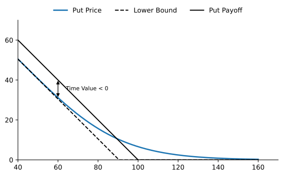
- Put-call parity and the fact that C \geq 0 implies that: P = C - S + K e^{-r T} \geq - S + K e^{-r T}
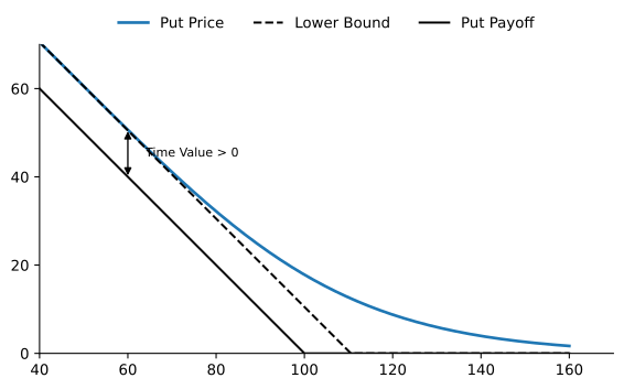
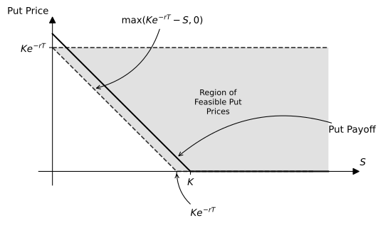
- Given that we also have P \geq 0, it must be the case that: P \geq \max(K e^{-r T} - S, 0)
- Also, the maximum amount of money one can lose by writing a European put is K, which in present value terms is equal to K e^{-r T}, implying that: P \leq K e^{-r T}
Feasible Prices for European Put Options
- The graph describes the region of feasible prices for European put options written on a non-dividend paying asset when the risk-free rate is positive.
Time Value of European Put Option (r > 0)
Summary
- We have the following bounds for European call and put options written on a non-dividend paying asset: \begin{aligned} \max(0, S - K e^{-r T}) \leq & C \leq S \\ \max(0, K e^{-r T} - S) \leq & P \leq K e^{-r T} \end{aligned}
Example 5
- The risk-free rate is r = 10\% per year with continuous compounding.
- Furthermore, assume that S = 50, K = 45, and T = 1.20.
- Let us compute the bounds for European call and put options.
- First, for the put option we have that: 0 = \max(45 e^{-0.10 \times 1.20} - 50, 0) \leq P \leq 45 e^{-0.10 \times 1.20} = 39.91
- Second, for the call option: 10.09 = \max(50 - 45 e^{-0.10 \times 1.20}, 0) \leq C \leq 50
Impact of Negative Interest Rates
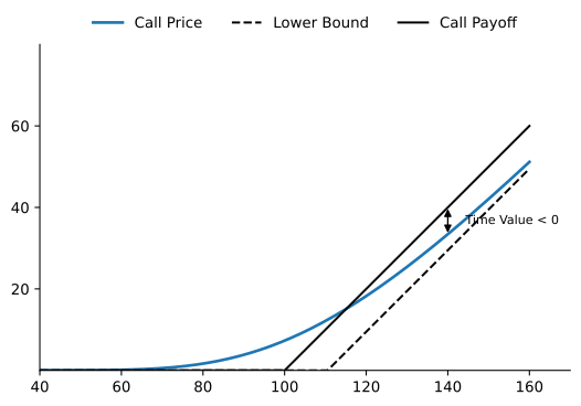
- During the last decade, interest rates in many countries became negative, even for maturities longer than 10 years.
- For a European call option, when r < 0 its lower bound is less than its intrinsic value, i.e., for a sufficiently high S the option will have negative time value and it might be optimal to early exercise an American call option.
- For put options, negative interest rates means that a European put option always has positive time value, i.e., it is not optimal to exercise early an American put option.
- Standard results that are usually taught in derivative courses get reversed!
Time Value of European Call Option (r < 0)
Time Value of European Put Option (r < 0)