Options on Assets Paying a Dividend Yield

Options, Futures and Derivative Securities

Lorenzo Naranjo

Spring 2026

General Framework

Pricing Formulas

• Consider an asset S that pays a continuous yield \textcolor{red}{\delta} and that follows a GBM under the risk-neutral measure: dS = (r-\textcolor{red}{\delta}) S dt + \sigma S dB^{*}
• The price of European call and put options with strike price K and time-to-maturity T are given by: \begin{aligned} C & = S \textcolor{red}{e^{-\delta T}} \operatorname{Φ}(d_{1}) - K e^{-r T} \operatorname{Φ}(d_{2}) \\ P & = K e^{-r T} \operatorname{Φ}(-d_{2}) - S \textcolor{red}{e^{-\delta T}} \operatorname{Φ}(-d_{1}) \end{aligned} where d_{1} = \frac{\ln(S/K) + (r - \textcolor{red}{\delta} + \frac{1}{2} \sigma^{2}) T}{\sigma \sqrt{T}} \text{ and } d_{2} = d_{1} - \sigma \sqrt{T}

Modeling Dividends

• It is usually convenient to model dividends as a percentage yield paid over time.
• We will denote the continuously-compounded dividend yield by \delta.
• Over each short interval \Delta t, the asset pays a dividend of \delta S_{t} \Delta t, known at time t.
• Therefore, if you purchase one unit of the asset at time t for S_{t}, the value of the portfolio at time t + \Delta t will be S_{t + \Delta t} + \delta S_{t} \Delta t.
• In practice, this is the approach used to model options on stock indices and currencies, although some practitioners also use it to model individual stocks as well.

Replicating A Derivative

• Consider a derivative H with maturity T written on an asset S that pays a continuous dividend yield \delta.
• The derivative can be replicated by buying N_{S} units of the stock and N_{Z} units of a bond with face value K and maturity T, respectively.
• If we call V the value of such replicating portfolio, we have that: V_{t} = N_{S, t} S_{t} + N_{Z, t} Z_{t}.
• At time t+\Delta t, the value of the replicating portfolio is: V_{t + \Delta t} = N_{S, t} (S_{t + \Delta t} + \delta S_{t} \Delta t) + N_{Z, t} Z_{t + \Delta t}, which implies that: \Delta V_{t} = N_{S, t} (\Delta S_{t} + \delta S_{t} \Delta t) + N_{Z, t} \Delta Z_{t}.

Replication in Continuous-Time

• As \Delta t \rightarrow 0, we have that: \begin{aligned} dV & = N_{S} (dS + \delta S dt) + N_{Z} dZ \\ & = N_{S} (dS + \delta S dt) + (N_{Z} Z) r dt \\ & = N_{S} (dS + \delta S dt) + r (V - N_{S} S) dt \\ & = \left(r V - (r - \delta) N_{S} S\right) dt + N_{S} dS \end{aligned}
• Also, Itô’s lemma implies that: dV = \left(\frac{1}{2} \sigma^{2} S^{2} \frac{\partial^{2} V}{\partial S^{2}} + \frac{\partial V}{\partial t}\right) dt + \textcolor{blue}{\frac{\partial V}{\partial S} dS} = \left(r V - (r - \delta) N_{S} S\right) dt + \textcolor{blue}{N_{S} dS}

The Risk-Neutral Process for the Underlying Asset

• Again, choosing N_{S} = \frac{\partial V}{\partial S} implies that: \frac{\partial V}{\partial t} + \frac{1}{2} \sigma^{2} S^{2} \frac{\partial^{2} V}{\partial S^{2}} + (r - \delta) S \frac{\partial V}{\partial S} - r V = 0 with boundary condition V_{T} = H_{T}.
• Using the same logic as before, we conclude that S follows a GBM under the risk-neutral measure given by: dS = (r - \delta) S dt + \sigma S dB^{*}

Pricing a Forward Contract

• We can use the risk-neutral approach to price a long forward contract with maturity T and forward price F. \begin{aligned} V_{t} & = e^{-r(T - t)} \operatorname{E}^{*}_{t}(S_{T} - F) \\ & = e^{-r (T - t)} (S_{t} e^{(r - \delta)(T - t)} - F) \\ & = S_{t} e^{-\delta (T - t)} - F e^{-r (T - t)} \end{aligned}
• The forward price F is determined such that at inception the value of the contract is zero: V = S e^{-\delta T} - F e^{-r T} = 0 \Rightarrow F = S e^{(r - \delta) T}
• The value of the long position, in general, will change over time.

Pricing a European Call Option

• As before, we can price a European call option written on the asset with maturity T and strike price K: \begin{aligned} C & = e^{-r T} \operatorname{E}^{*}\left((S_{T} - K) 1\kern-0.25em\text{l}_{\{S_{T} > K\}} \right) \\ & = e^{-r T} \operatorname{E}^{*}\left(S_{T} 1\kern-0.25em\text{l}_{\{S_{T} > K\}} \right) - e^{-r T} \operatorname{E}^{*}\left(K 1\kern-0.25em\text{l}_{\{S_{T} > K\}} \right) \\ & = S e^{-\delta T} \operatorname{Φ}(d_{1}) - K e^{-r T} \operatorname{Φ}(d_{2}) \end{aligned} where \begin{aligned} d_{1} & = \frac{\ln(S/K) + (r - \delta + \frac{1}{2} \sigma^{2}) T}{\sigma \sqrt{T}} \\ d_{2} & = d_{1} - \sigma \sqrt{T} \end{aligned}

Call Premium vs. Spot Price

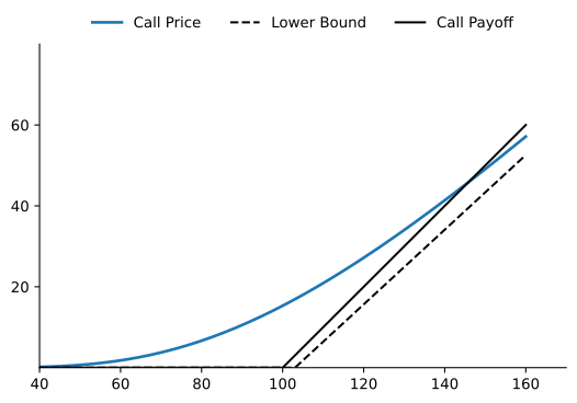
The figure displays the Black-Scholes call premium C(S) where r = 0.05, \delta = 0.08, \sigma = 0.45, T = 1 and K = 100. It also shows the call option payoff given by \max(S - K, 0) and the lower bound for a European call given by \max(S e^{-\delta T} - K e^{-r T}, 0).

Pricing a European Put Option

• Consider now a European put option with the same characteristics as the previous call.
• According to put-call parity, it must be the case that: C - P = S e^{-\delta T} - K e^{-r T}
• Hence, \begin{aligned} P & = C - (S e^{-\delta T} - K e^{-rT}) \\ & = S e^{-\delta T} \operatorname{Φ}(d_{1}) - K e^{-r T} \operatorname{Φ}(d_{2}) - (S e^{-\delta T} - K e^{-rT}) \\ & = K e^{-r T} (1 - \operatorname{Φ}(d_{2})) - S e^{-\delta T} (1 - \operatorname{Φ}(d_{1})) \\ & = K e^{-r T} \operatorname{Φ}(-d_{2}) - S e^{-\delta T} \operatorname{Φ}(-d_{1}) \end{aligned}

Put Premium vs. Spot Price

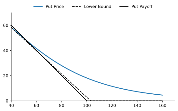
The figure displays the Black-Scholes put premium P(S) where r = 0.05, \delta = 0.08, \sigma = 0.45, T = 1 and K = 100. It also shows the put option payoff given by \max(K - S, 0) and the lower bound for a European put given by \max(K e^{-r T} - S e^{-\delta T}, 0).

Example 1 A stock that pays a continuous dividend yield of 8% currently trades for $100. The instantaneous volatility of returns is 30% per year and the risk-free rate is 5% per year, continuously compounded and constant for all maturities. Consider ATM call and put options written on the stock with maturity 10 months. Then, \begin{aligned} d_{1} & = \frac{\ln(100/100) + (0.05 - 0.08 + 0.5(0.30)^{2})(10/12)}{0.30\sqrt{10/12}} = 0.0456 \\ d_{2} & = 0.0456 - 0.30\sqrt{10/12} = -0.2282 \end{aligned} Therefore, \operatorname{Φ}(d_{1}) = 0.5182 and \operatorname{Φ}(d_{2}) = 0.4097, which implies that: \begin{aligned} C & = 100e^{-0.08(10/12)}(0.5182) - 100e^{-0.05(10/12)}(0.4097) = \$9.18 \\ P & = 100e^{-0.05(10/12)}(1 - 0.4097) - 100e^{-0.08(10/12)}(1 - 0.5182) = \$11.54 \end{aligned}

Delta of European Call and Put Options

• For an asset that pays a continuous dividend yield \delta, we have that for a European call option: \frac{\partial C}{\partial S} = e^{-\delta T} \Phi(d_{1})
• We can see that if \delta > 0, the number of shares required to hedge the call is lower than in the case of a non-dividend paying asset.
  • The shares that you buy to hedge the call grow over time at the rate \delta, which means that you need to buy less.
• Similarly, for a European put option we have that: \frac{\partial P}{\partial S} = - e^{-\delta T} \Phi(-d_{1})

Example 2 In the previous example, we found that \operatorname{Φ}(d_{1}) = 0.5182 and \operatorname{Φ}(d_{2}) = 0.4097. Hence, \begin{aligned} \frac{\partial C}{\partial S} & = e^{-0.08(10/12)} (0.5182) = 0.4848 \\ \frac{\partial P}{\partial S} & = - e^{-0.08(10/12)} (1 - 0.5182) = -0.4507 \end{aligned} This means that an OTC dealer who sells a call option needs to buy 0.4848 units of the asset while borrowing 100 e^{-0.05 (10/12)} (0.4097) = \$39.30 at the risk-free rate.

To hedge a put option, the dealer needs to short-sell 0.4507 units of the asset and invest 100 e^{-0.05 (10/12)} (1 - 0.4097) = \$56.62 in the money-market account.

Options on Stock Indices

Options on Stock Indices

• Most stock indices such as the S&P 500 (SPX) do not reinvest their dividends.
• Hence, to replicate an option written on the index we can use a portfolio of stocks that mimics the value of the index and that will pay a dividend yield over time.
• We will assume that the replicating portfolio exactly matches the composition of the index at any point in time so that S_{t} represents both the value of the index and of the tracking portfolio.

SPX Options

• One of the most liquid option contracts in the world.
• Characteristics:
  • European style exercise
  • Cash settled
  • Each contract is written on 100 times the value of the index
    
• There are also mini-SPX index options written over XSP which is an index 10 times smaller than SPX.
• More information can be found at https://cdn.cboe.com/resources/spx/spx-fact-sheet.pdf

Example 3 The SPX index is currently at 4,251, has a dividend yield of 1.33% per year and an instantaneous volatility of 17% per year. The risk-free rate is 3% per year, continuously compounded and constant for all maturities. Say we want to compute the price of an SPX call option contract with maturity 3 months and strike 4,300. Then, \begin{aligned} d_{1} & = \frac{\ln(4251/4300) + (0.03 - 0.0133 + 0.5(0.17)^{2})(3/12)}{0.17\sqrt{3/12}} = -0.0432 \\ d_{2} & = -0.0432 - 0.17\sqrt{3/12} = -0.1282 \end{aligned} Hence, \operatorname{Φ}(d_{1}) = 0.4828 and \operatorname{Φ}(d_{2}) = 0.4490, which implies that: \begin{aligned} C = 4,251 e^{-0.0133(3/12)}(0.4828) - 4,300 e^{-0.03(3/12)}(0.4490) = \$129.193 \end{aligned} Therefore, a standard SPX call option contract should cost $12,919.30, whereas a mini-SPX call option contract should trade for $1,291.93.

Options on Currencies

Currencies as Assets Paying a Dividend Yield

• S is the price of one unit of the base currency in units of the quote currency, e.g., dollars per euro for EUR/USD.
• r is the interest rate of the quote currency and r_{f} the interest rate of the base currency.
• A deposit in the base currency earns r_{f}, exactly as the index earns its dividend yield \delta.
  • Holding the deposit is riskless, so the replication argument goes through with \delta = r_{f}.
• Under the risk-neutral measure: dS = (r - r_{f}) S dt + \sigma S dB^{*}
• The forward price F = S e^{(r - r_{f}) T} is covered interest parity.

Calls and Puts on Currencies

• A call in one currency’s terms is a put in the other’s.
• A call on EUR/USD with maturity 1 year, strike $1.25, and notional €1 million is, for a European investor, a put on USD/EUR with strike €0.80 and notional $1.25 million.
• Standard practice names both currencies: a EUR call / USD put.

Garman-Kohlhagen Model

• Replacing \delta by r_{f} in the Black-Scholes formulas gives the model of Garman and Kohlhagen (1983): \begin{aligned} C & = S e^{-r_{f} T} \operatorname{Φ}(d_{1}) - K e^{-r T} \operatorname{Φ}(d_{2}) \\ P & = K e^{-r T} \operatorname{Φ}(-d_{2}) - S e^{-r_{f} T} \operatorname{Φ}(-d_{1}) \end{aligned} where d_{1} = \frac{\ln(S/K) + (r - r_{f} + \frac{1}{2}\sigma^{2})T}{\sigma\sqrt{T}} \quad \text{and} \quad d_{2} = d_{1} - \sigma\sqrt{T}
• Put-call parity: C - P = S e^{-r_{f} T} - K e^{-r T}.
• An option with strike equal to the forward price, K = F, is at-the-money-forward (ATMF), and then C = P.

Example 4 The EUR/USD spot rate is $1.25. The volatility of the exchange rate is 12% per annum, the USD risk-free rate is 3%, and the EUR risk-free rate is 1%. Consider a 6-month EUR call / USD put and a EUR put / USD call, both with strike $1.28. Then, \begin{aligned} d_{1} & = \frac{\ln(1.25/1.28) + (0.03 - 0.01 + \frac{1}{2}(0.12)^{2})(0.5)}{0.12\sqrt{0.5}} = -0.1192, \\ d_{2} & = -0.1192 - 0.12\sqrt{0.5} = -0.2041. \end{aligned} Hence, \operatorname{Φ}(d_{1}) = 0.4525 and \operatorname{Φ}(d_{2}) = 0.4191, and \begin{aligned} C & = 1.25\, e^{-0.01(0.5)} (0.4525) - 1.28\, e^{-0.03(0.5)} (0.4191) = \$0.0343, \\ P & = 1.28\, e^{-0.03(0.5)} (1 - 0.4191) - 1.25\, e^{-0.01(0.5)} (1 - 0.4525) = \$0.0515. \end{aligned} As a check, C - P = -\$0.0172 = 1.2438 - 1.2609.

From Spot to Forward

• Since F = S e^{(r - r_{f}) T}, the same formulas can be written with the forward rate in place of S and r_{f}.
• That form is Black’s model, which we develop in Options on Futures.

References

Garman, Mark B., and Steven W. Kohlhagen. 1983. “Foreign Currency Option Values.” Journal of International Money and Finance 2 (3): 231–37.