Multiple Periods

Options, Futures and Derivative Securities

Lorenzo Naranjo

Spring 2026

Binomial Trees with Multiple Periods

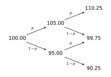
Example: Two-Period Binomial Tree

Note: Each period the asset can go up or down by 5%.

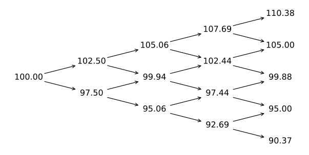
Example: Four-Period Binomial Tree

Note: Each period the asset can go up or down by 2.5%.

Recombinant Trees

• In the previous examples, going first up and then down is the same as going first down and then up.
• A recombinant tree is obtained whenever u and d are kept constant in each node of the tree.
  • The up and down moves need not be symmetric: the tree recombines even if d \neq 1/u.
• When this happens we say that the tree recombines.
  • Recombinant trees are very useful in modeling the stochastic behavior of financial assets because the number of nodes increases linearly with the number of periods, i.e after n periods there are n + 1 possible nodes.
  • If the tree does not recombine then the number of nodes increases exponentially, i.e. after n periods there are 2^{n} possible nodes.

Example

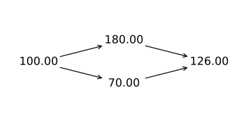
• Is it the same for an asset to go up by 80% and then down by 30%, compared to first go down by 30% and then go up by 80%?
• Consider an asset whose current price is $100.

• The tree recombines because multiplication is commutative: S_{ud} = 100 \times 1.80 \times 0.70 = 100 \times 0.70 \times 1.80 = S_{du}

Pricing Options with Multiple Periods

The Two Period Binomial Model

• We now extend the economy to two periods
• The stock price is S
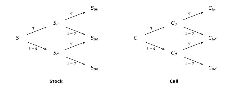
• Each period the stock price goes up by u or goes down by d with risk-neutral probabilities q and 1 - q, respectively
• Therefore:
  • S_{u} = S \times u and S_{d} = S \times d
  • S_{uu} = S_{u} \times u, S_{ud} = S_{u} \times d = S_{d} \times u = S_{du} and S_{dd} = S_{d} \times d
• A call option expiring at T and strike K trades at C
• The time-step is then \Delta t = T / 2

Two Period Tree for the Stock and Call Option

Pricing a Call Option

• The call price at expiration is the intrinsic value of the option: C_{i} = \max(S_{i} - K, 0) where i represents all the nodes at expiration.
• In all other nodes of the tree it must be the case that: C_{i} = \left( q C_{iu} + (1 - q) C_{id} \right) e^{-r \Delta t}
• We can work backwards to find the price of the option today.

Dynamic Replication

• At each node, the option pays one of two values next period, so the one-period replication argument applies node by node.
• The replicating portfolio changes as we move through the tree:
  • Today: N_{S} = (C_{u} - C_{d})/(S_{u} - S_{d}) shares.
  • After an up move: N_{S}^{u} = (C_{uu} - C_{ud})/(S_{uu} - S_{ud}) shares.
  • After a down move: N_{S}^{d} = (C_{ud} - C_{dd})/(S_{ud} - S_{dd}) shares.
• The strategy is self-financing: at each node, the portfolio is worth exactly what the new hedge costs.
• Replication in a multi-period tree is dynamic: the hedge is adjusted every period.

Example 1

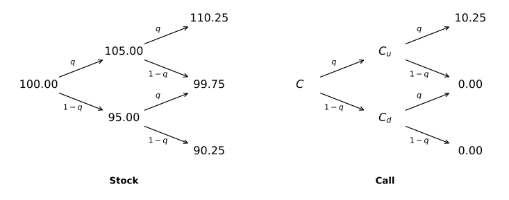
• Let us price a European call option written on a non-dividend paying stock using a two-step binomial model.
• The current stock price is $100, and it can go up or down by 5% each period for two periods.
• Each period represents 3-months, i.e. \Delta t = 0.25.
• The risk-free rate is 6% per year (continuously compounded).
• Compute the price of a European call option with maturity 6 months and strike $100.

Two Period Tree for the Stock and Call Option

Computing the Risk-Neutral Probabilities

• The risk-neutral probability of an up-move is then q = \frac{e^{r \Delta t} - d}{u - d} = \frac{e^{0.06 \times 0.25} - 0.95}{1.05 - 0.95} = 0.6511.
• The risk-neutral probability of a down-move is just 1 - q = 0.3489.

Pricing the European Call Option

• We then compute the price of the call in 3-months if the stock price moves up: C_{u} = \left( 10.25 \times q + 0 \times (1 - q) \right) e^{-0.06 \times 0.25} = \$6.57
• Next, we compute the price of the call in 3-months if the stock price moves down: C_{d} = \left( 0 \times q + 0 \times (1 - q) \right) e^{-0.06 \times 0.25} = \$0
• Finally, we compute the price of the call: C = \left( 6.57 \times q + 0 \times (1 - q) \right) e^{-0.06 \times 0.25} = \$4.22

Hedging the Call

• Today the replicating portfolio holds N_{S} = (6.57 - 0)/(105 - 95) = 0.657 shares.
• If the stock goes up, rebalance to N_{S}^{u} = (10.25 - 0)/(110.25 - 99.75) = 0.976 shares: the call is likely to finish in the money.
• If the stock goes down, the call can no longer pay off: sell all the shares, N_{S}^{d} = 0.

Pricing a European Put Option

• We can use the risk-neutral probabilities to price a European put with the same characteristics. \begin{aligned} P_{u} & = \left( 0 \times q + 0.25 \times (1 - q) \right) e^{-0.06 \times 0.25} = \$0.09 \\ P_{d} & = \left( 0.25 \times q + 9.75 \times (1 - q) \right) e^{-0.06 \times 0.25} = \$3.51 \\ P & = \left( 0.09 \times q + 3.51 \times (1 - q) \right) e^{-0.06 \times 0.25} = \$1.26 \end{aligned}
• Put-call parity confirms it: P = C - S + K e^{-r T} = 4.22 - 100 + 100 e^{-0.06 \times 0.5} = \$1.26.

Making the Tree Consistent with Observed Volatility

• It is possible to relate the up and down movements to the risk-neutral volatility observed in the market.
• It can be shown that over an interval \Delta t, the choice u = e^{\sigma \sqrt{\Delta t}} and d = 1 / u produce a binomial model consistent with the Black-Scholes model of a Geometric Brownian Motion (GBM).
• Note that in this case u \times d = 1, so the horizontal center of the tree stays constant (every other period).
• The risk-neutral drift, however, is incorporated into the risk-neutral probabilities.

A Shortcut for European Options

• A European option can be priced directly from its payoffs at maturity.
• With n periods, the stock price after n - i up-moves and i down-moves is S_{T}(i) = S u^{n - i} d^{i}, \quad i = 0, \ldots, n
• The total risk-neutral probability of that node is Q(i) = \binom{n}{i} q^{n - i} (1 - q)^{i}
• Therefore, C = e^{-r T} \sum_{i = 0}^{n} Q(i) \max(S_{T}(i) - K, 0), \quad P = e^{-r T} \sum_{i = 0}^{n} Q(i) \max(K - S_{T}(i), 0)
• American options need the full tree, since early exercise must be checked at every node.

Pricing a European Call Option Using Five Periods

• In this example we price a 6-month European call option with strike price $135 written on a non-dividend paying stock that currently trades at $132 and whose volatility of stock returns is 35% per year.
• The interest rate is 3% per year with continuous compounding.
• We will use a 5-period binomial tree.
• Therefore, we have that
  • T = 6/12 = 0.5
  • \Delta t = T / 5 = 0.1
  • u = e^{0.35 \sqrt{0.1}} = 1.1170
  • d = 1/1.1170 = 0.8952

Binomial Tree for the Stock

• It’s convenient and efficient in this case to write the tree as a lower triangle.

Time	0	0.1	0.2	0.3	0.4	0.5
Stock	132	147.45	164.71	183.98	205.52	229.57
		118.17	132.00	147.45	164.71	183.98
			105.79	118.17	132.00	147.45
				94.70	105.79	118.17
					84.78	94.70
						75.90

Pricing the Call

• The risk-neutral probability of an up-move is given by: \begin{aligned} q = \frac{e^{0.03 \times 0.1} - 0.8952}{1.1170 - 0.8952} = 0.4859 \end{aligned}
• We can now price the call as follows.

Time	0	0.1	0.2	0.3	0.4	0.5
Call	13.16	21.23	33.18	49.79	70.92	94.57
		5.60	10.06	17.68	30.11	48.98
			1.42	2.92	6.03	12.45
				0.00	0.00	0.00
					0.00	0.00
						0.00

Checking with the Shortcut

• Only the three highest nodes pay off, so C = e^{-0.03 \times 0.5} \left( q^{5} \times 94.57 + 5 q^{4} (1 - q) \times 48.98 + 10 q^{3} (1 - q)^{2} \times 12.45 \right) = \$13.16
• The shortcut gives the same price as working backwards through the tree.

Assets Paying a Dividend Yield

Binomial Pricing with a Dividend Yield

• Holding the asset earns the yield \delta, so its forward price over the next period is S e^{(r - \delta) \Delta t}.
• The only change to the tree is the risk-neutral probability, which must reproduce that forward price.
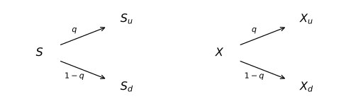
• Over the next period \Delta t the asset price can go up to S_{u} = S u or down to S_{d} = S d, and a derivative X pays X_{u} or X_{d}, respectively.

Risk-Neutral Pricing with a Dividend Yield

• The risk-neutral probability of an up-move is: q = \frac{e^{(r - \delta) \Delta t} - d}{u - d}
• The price of the derivative is then: X = (q X_{u} + (1 - q) X_{d}) e^{-r \Delta t}
• A share bought today grows to e^{\delta \Delta t} shares, so the hedge buys fewer shares up front: N_{S} = \frac{X_{u} - X_{d}}{S_{u} - S_{d}} e^{-\delta \Delta t}
• The calibration u = e^{\sigma \sqrt{\Delta t}} and d = 1/u carries over unchanged.

Example 2

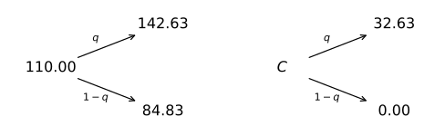
• Suppose that S = 110, r = 5\%, \delta = 3\%, \sigma = 30\%, K = 110, T = 9 months.
• Using a one-period binomial tree, let’s compute the no-arbitrage price of a European call option.
• The binomial trees for the asset and the call are as follows:

Example 2 (cont’d)

• The risk-neutral probability of an up-move is q = \frac{110 e^{(0.05 - 0.03) \times 9/12} - 84.83}{142.63 - 84.83} = 0.4642
• The price of the call is then given by C = (32.63 q + 0 (1 - q)) e^{-0.05 \times 9/12} = 14.59