Interest Rates

Options, Futures and Derivative Securities

Lorenzo Naranjo

Spring 2026

Introduction

Interest Rates and Derivatives

• The pricing of financial assets is always relative to some benchmarks that we believe are well priced.
• In order to compare cash flows occurring at different points in time, we use risk-free bonds as the relevant benchmarks.
• Unfortunately, real financial markets are rarely fully integrated, so the landscape of interest rates is varied and complex.
• Moreover, when pricing options and other derivatives, it is common both by academics and practitioners to use continuous compounding to discount riskless cash flows.

Example 1

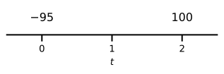
• Consider a zero-coupon bond that pays for certain $100 in 2 years.
• The bond today costs $95.

• The fact that $100 paid in two years costs today $95 can also be expressed as a percentage rate of return per year. 95 (1 + r)^{2} = 100 \Rightarrow r = \left( \frac{100}{95} \right)^{1/2} - 1 = 2.60\%.
• In other words, the implicit interest rate paid by the 2-year zero coupon bond is 2.60% per year compounded annually.

Example 1 (continued)

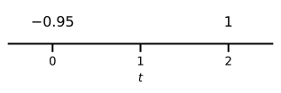
• This means that every dollar paid for certain in two years today costs $0.95.

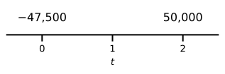
• Thus, a bond that pays for certain $50,000 in two years today should cost 0.95 \times 50{,}000 = \$47{,}500.

An Arbitrage Example

• What if this new bond trades for a different price, say $47,000?
• Then there would be an arbitrage opportunity.
• These two strategies pay the same:
  • 500 bonds paying $100 in two years
  • 1 bond paying $50,000 in two years
• How to profit?
  • Buy the bond with face value $50,000 expiring in two years.
  • Sell 500 bonds with face value $100 expiring at the same date.
    
• This long-short strategy provides today with a positive cash-flow of $500 and is fully hedged in two years.

Different Types of Interest Rates

Treasury Rates

• The United States government through the Department of the Treasury issues Bills, Notes and Bonds to finance government activities.
• Treasury bonds are usually perceived as risk-free, i.e. no risk of default.
• Despite the size of the U.S. Treasury market, the demand for Treasury securities often surpasses its supply.
• For this reason, the yield-to-maturity (YTM) of Treasury bonds might be lower than the rate of a fully collateralized loan.
• Therefore, Treasury rates are commonly not used as benchmark rates to price derivative securities.

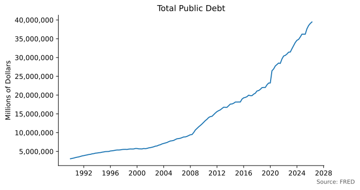
U.S. Public Debt

LIBOR

• The London Interbank Offered Rate (LIBOR) has been at the heart of the financial system for many decades.
• For all this time, LIBOR has provided a reference for pricing derivatives, loans and securities.
• Large corporate loans used to be indexed to LIBOR.
• Since many borrowers liked to pay a fixed rate, one of the most important derivatives that used LIBOR as a reference rate were interest rate swaps.
• LIBOR is no longer used and in the U.S. it has been replaced with SOFR.

OIS and Overnight Rates

• In the United States, banks hold reserve balances at the Federal Reserve and lend them to each other overnight in the federal funds market.
• Reserve requirements have been zero since March 2020, but institutions still trade reserves to manage their liquidity.
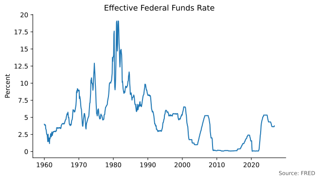
• The volume-weighted median rate of these overnight loans is termed the (EFFR).
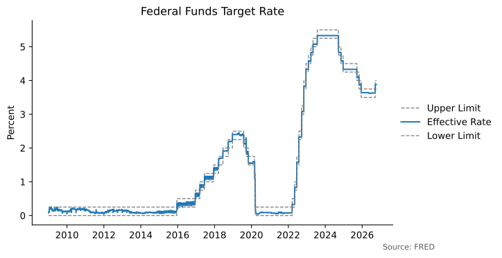
• When the Federal Reserve determines the , they implement their policy by making sure that the EFFR is close every day to their target.
• An overnight indexed swap (OIS) is an over-the-counter financial contract in which one party pays the compounded EFFR over a certain period, say three months, in exchange for a fixed payment.

Evolution of the Effective Federal Funds Rate

Federal Reserve Interest Rate Policy

SOFR and Repo Rates

• In a repurchase agreement or repo, a financial institution or trader sells some securities to a counterparty with the agreement to repurchase them back later for a slightly higher price.
• The implicit interest rate in this transaction is the repo rate.
• Unlike LIBOR and the EFFR, repo rates are secured borrowing rates.
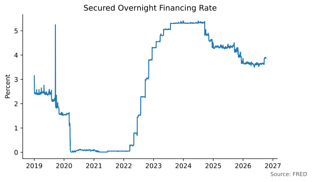
• The volume-weighted median rate of overnight repo transactions backed by Treasury securities is called the (SOFR).
• U.S. regulators told banks to stop writing new LIBOR contracts after 2021, and SOFR has since replaced LIBOR USD.
• Given its close connection to secured overnight borrowing in a deep and liquid market, SOFR is the benchmark risk-free rate we will use when pricing futures, forwards, and options.

Secured Overnight Financing Rate (SOFR)

Compounding Frequencies

Compounding Multiple Times per Year

• Suppose you have $100 to invest for a year and the interest rate is 10%.
• It makes a difference how often you compound the interest.
• As you compound more often you earn more interest-on-interest.

Compounding Frequency	Future Value
Annual	100(1.10)=\$110.00
Semi-Annual	100(1.05)^{2}=\$110.25
Quarterly	100\left(1+\frac{0.10}{4}\right)^{4}=\$110.38
Monthly	100\left(1+\frac{0.10}{12}\right)^{12}=\$110.47
Daily	100\left(1+\frac{0.10}{365}\right)^{365}=\$110.52

Compounding in the Limit

• It turns out that there is a limit to the compounding operation we just did: \lim_{n\rightarrow\infty} 100\left(1+\frac{0.10}{n}\right)^{n} = 100e^{0.10} = \$110.52.
• We call this operation continuous compounding, and you can see that compounding daily is already a pretty good approximation of it.
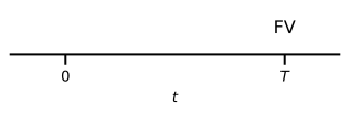
• In general, if we denote by r the continuously-compounded interest rate, the relationship between present value (PV) and future value (FV) is given by: \text{FV}=\text{PV}e^{rT} \Longleftrightarrow \text{PV}=\text{FV}e^{-rT}

A Note on Exponentials

• In the previous expression e^{x} = \exp(x) is called the exponential function.
• In a spreadsheet, for example, if you want to compute 100 e^{0.10} you need to type =100*exp(0.10), which will return 110.52.
• If, on the other hand, you want to know which rate r gives you a future value of $110 over a year if you invest $100 and the rate is compounded continuously, then we need to solve: 110 = 100 e^{r}, which is the same as solving for r in e^{r} = 1.10.
• The natural logarithm function allows us to solve for r, that is e^{r} = 1.10 \Leftrightarrow r = \ln(1.10) = 9.53\%.

Converting Between Compounding Conventions

• To convert a rate r_m compounded m times per year to a rate r_n compounded n times per year, equate future values: \left(1 + \frac{r_m}{m}\right)^{m} = \left(1 + \frac{r_n}{n}\right)^{n}.
• To convert to a continuously-compounded rate r_c, take the limit n \to \infty: \left(1 + \frac{r_m}{m}\right)^{m} = e^{r_c} \Rightarrow r_c = m \ln\!\left(1 + \frac{r_m}{m}\right).

Effective Annual Rate (EAR)

• In the previous slide we saw that 100 \times 1.10 = 110 = 100e^{0.0953}.
• Therefore 10% per year compounded annually is the same as 9.53% per year compounded continuously because it gives us the same amount of money after a year.
• We can also say that 9.53% per year compounded continuously is equivalent to an effective annual rate (EAR) of 10% per year.

Example 2: Pricing a Zero-Coupon Bond

• A zero-coupon bond pays its principal or face-value (FV) at maturity but makes no intermediate payments.

• The continuously-compounded interest rate is 8% per year.
• Consider a zero-coupon risk-free bond with face value $1,000 and expiring in seven months.
• The price of the bond is: B = 1000e^{-0.08 \times 7/12} = \$954.41.

Example 3: Pricing a Coupon-Bond

• A coupon-bond pays a periodic amount (C) either every year or every six months, and its principal or face-value (FV) at maturity.

• The continuously-compounded interest rate is 6% per year.
• Consider a bond that pays coupons of 4% every year over a notional of $1,000 and expiring in four years.
• The price of the bond is: B = 40e^{-0.06 \times 1} + 40e^{-0.06 \times 2} + 40e^{-0.06 \times 3} + 1040e^{-0.06 \times 4} = \$924.65.

Zero Rates

Where Do Zero Rates Come From?

• In general, the interest rate for different maturities is not the same.
• The collection of interest rates for different maturities is called the term-structure of interest rates.
• The price of a zero-coupon bond is determined by discounting its face-value at the relevant interest rate.
• For a given maturity \tau, the \tau-year zero rate, denoted by r(\tau), is the interest rate that gives the correct \tau-year zero-coupon bond price Z_{\tau}.
• If r(\tau) is a continuously-compounded rate we must have: Z_{\tau} = F e^{-r(\tau) \tau}.

Example 4

• You have the following information for zero rates expressed per year with continuous compounding.

Maturity (months)	1	3	6	9	12
Zero Rate (%)	6.0	6.4	6.6	6.8	7.0

• Consider a zero-coupon risk-free bond with face value $1,000 and expiring in 9 months.
• The price of the bond is: B = 1000e^{-0.068 \times 9/12} = \$950.28.