The Impact of Dividends
Options, Futures and Derivative Securities
Lorenzo Naranjo
Spring 2026
Assets Paying Cash Dividends
Put-Call Parity with Dividends
- For European options written on dividend paying stocks, the put-call parity is modified as follows: C - P = S - D - K e^{-r T} where D is the present value of dividends paid during the life of the option.
- In order to derive this expression we will proceed as before by trying to build a covered call in two different ways.
Building a Covered Call
- Use the same two strategies as for non-dividend paying stocks.
- Strategy A: Long stock and short call \begin{align*} \text{Cost} & = S - C \\ \text{Payoff} & = \begin{cases} S_{T} + \textit{FV}(D) & \text{if $S_{T} \leq K$} \\ K + \textit{FV}(D) & \text{if $S_{T} > K$} \end{cases} \end{align*}
- Strategy B: Long bond and short put \begin{align*} \text{Cost} & = K e^{-r T} - P \\ \text{Payoff} & = \begin{cases} S_{T} & \text{if $S_{T} \leq K$} \\ K & \text{if $S_{T} > K$} \end{cases} \end{align*}
- Both strategies no longer have the same payoff at maturity because the stock pays dividends.
Adjusting Strategy A
- Strategy A: Long stock, borrow D and short call \begin{align*} \text{Cost} & = S - D - C \\ \text{Payoff} & = \begin{cases} S_{T} & \text{if $S_{T} \leq K$} \\ K & \text{if $S_{T} > K$} \end{cases} \end{align*}
- Strategy B: Long bond and short put \begin{align*} \text{Cost} & = K e^{-r T} - P \\ \text{Payoff} & = \begin{cases} S_{T} & \text{if $S_{T} \leq K$} \\ K & \text{if $S_{T} > K$} \end{cases} \end{align*}
- Note that in A we use the dividends, reinvested at r, to repay the loan and generate the same payoff as in B.
Example 1
- Suppose that S = 110, r = 5\%, K = 110, T = 9 months, and C = 13.30.
- The stock is expected to pay dividends of $2 in 6 months, and $2.5 in 1 year.
- What should be the no-arbitrage price of a European put with the same strike and maturity as the European call?
- The present value of the relevant dividends is: D = 2 e^{-0.05 \times 6/12} = 1.95
- Then, according to put-call parity we should have that: P = 13.30 - 110 + 1.95 + 110 e^{-0.05 \times 9/12} = 11.20
Example 2
- What if in the previous example everything stays the same, but you find that the put trades for $11?
- Then we have an arbitrage opportunity since the put is relatively cheap compared to what it should trade.
- Hence, we should buy the put and sell the synthetic put. Note that the stock will pay a dividend of $2 in six months that can be used to pay the loan at that time.
Example 2 (cont’d)
| Transactions | T = 0 | T = 6/12 | T = 9/12, S_{T} \leq 110 | T = 9/12, S_{T} > 110 |
|---|---|---|---|---|
| Long put | -11.00 | 0 | 110 - S_{T} | 0 |
| Short call | 13.30 | 0 | 0 | -(S_{T} - 110) |
| Long stock | -110.00 | 2 | S_{T} | S_{T} |
| Borrow D | 1.95 | -2 | 0 | 0 |
| Short bond | 105.95 | 0 | -110 | -110 |
| Total | 0.20 | 0 | 0 | 0 |
Lower Bound on European Options with Cash Dividends
- With dividends, we modify the lower bounds on European call and put options as follows: \begin{align*} C & \geq \max(S - D - K e^{-r T}, 0) \\ P & \geq \max(K e^{-r T} - S + D, 0) \end{align*}
- As for the case with no dividends, these results are a consequence of put-call parity and the fact the option premium is never negative.
Example 3
- Suppose that you have S = 110, r = 5\%, K = 110, and T = 9 months.
- The stock is expected to pay dividends of $2 and $2.5, in six and twelve months, respectively.
- The previous result implies that: C \geq \max(110 - 2 e^{-0.05 \times 6/12} - 110 e^{-0.05 \times 0.75}, 0) = 2.10
- Note that we only include the dividend paid in 6 months since the maturity of the option is 9 months.
- Also note that the bound is lower than the bound for an otherwise equivalent option written on a non-dividend paying stock.
- For European options you can only purchase the stock at maturity and therefore you miss the dividend paid in 6 months.
Upper Bound on European Options with Cash Dividends
- Since the payoffs of strategies A and B described above are positive, the cost of both strategies must be positive.
- Therefore, if the asset pays cash dividends, the upper bounds on European call and put options are as follows: \begin{align*} C & \leq S - D \\ P & \leq K e^{-r T} \end{align*}
Example 4
- Suppose that you have S = 110, r = 5\%, K = 110, and T = 9 months.
- The stock is expected to pay dividends of $2 and $2.5, in six and twelve months, respectively.
- The previous result implies that: C \leq 110 - 2 e^{-0.05 \times 6/12} = 108.05
- Hence, no matter how high the volatility is on this European call option with strike $110 and maturity 9 months, its premium must be less than $108.05.
Assets Paying a Dividend Yield
The Dividend Yield
- There are many assets that pay dividends continuously, like a currency, or that can be modeled as such, like a stock index.
- In these cases it is convenient to model dividends as a percentage yield paid over time.
- We will denote the continuously-compounded dividend yield by \delta.
- Over each short interval \Delta t, the asset pays a dividend of \delta S_{t} \Delta t.
- Therefore, the dividend yield can be seen as the units of the asset growing over time at the rate \delta.
- In practice, this is the approach used to model options on stock indices and currencies, although some practitioners also use it to model individual stocks as well.
Put-Call Parity with a Dividend Yield
- For European options written on assets paying a dividend yield, the put-call parity is modified as follows: C - P = S e^{-\delta T} - K e^{-r T} where \delta is the dividend yield paid continuously by the asset during the life of the option.
- In order to derive this expression we will proceed as before by trying to build a covered call in two different ways.
Two Strategies with the Same Payoff
- Strategy A: Long e^{-\delta T} units of the asset and short call \begin{align*} \text{Cost} & = S e^{-\delta T} - C \\ \text{Payoff} & = \begin{cases} S_{T} & \text{if $S_{T} \leq K$} \\ K & \text{if $S_{T} > K$} \end{cases} \end{align*}
- Strategy B: Long bond and short put \begin{align*} \text{Cost} & = K e^{-r T} - P \\ \text{Payoff} & = \begin{cases} S_{T} & \text{if $S_{T} \leq K$} \\ K & \text{if $S_{T} > K$} \end{cases} \end{align*}
- Note that in A the asset grows at the rate \delta, so the total number of “units” of the asset at maturity is e^{-\delta T} e^{\delta T} = 1.
Example 5
- Suppose that S = 110, r = 5\%, \delta = 3\%, K = 110, T = 9 months, and C = 13.30.
- What should be the no-arbitrage price of a European put with the same strike and maturity as the European call?
- According to put-call parity we should have that a European put with the same strike and maturity as the call should cost: P = 13.30 - 110 e^{-0.03 \times 9/12} + 110 e^{-0.05 \times 9/12} = 11.70.
Example 6
- What if in the previous example everything stays the same, but you find that the put trades for $11?
- Then we have an arbitrage opportunity since the put is relatively cheap compared to what it should trade.
- Hence, we should buy the put and sell the synthetic put.
| Transactions | T = 0 | T = 9/12, S_{T} \leq 110 | T = 9/12, S_{T} > 110 |
|---|---|---|---|
| Long put | -11.00 | 110 - S_{T} | 0 |
| Short call | 13.30 | 0 | -(S_{T} - 110) |
| Long e^{-\delta T} units of asset | -107.55 | S_{T} | S_{T} |
| Short bond | 105.95 | -110 | -110 |
| Total | 0.70 | 0 | 0 |
Lower Bound on European Options with Dividend Yields
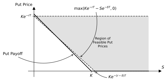
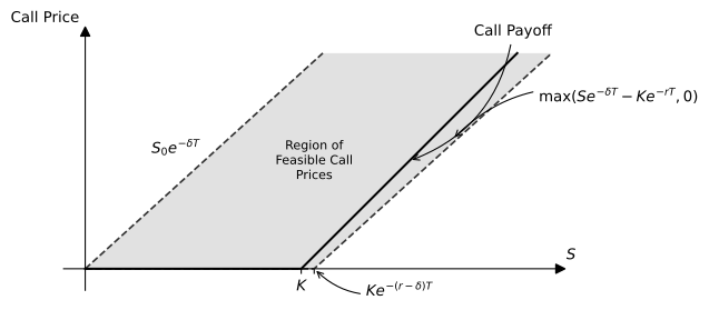
- If the asset pays a dividend yield, we modify the lower bounds on European call and put options as follows: \begin{align*} C & \geq \max(S e^{-\delta T} - K e^{-r T}, 0) \\ P & \geq \max(K e^{-r T} - S e^{-\delta T}, 0) \end{align*}
- As for the case with no dividends, these results are a consequence of put-call parity and the fact the option premium is never negative.
Example 7
- Suppose that you have S = 110, r = 5\%, \delta = 3\%, K = 110, and T = 9 months.
- The previous result implies that: C \geq \max(110 e^{-0.03 \times 9/12} - 110 e^{-0.05 \times 9/12}, 0) = 1.60
- Hence, no matter how low the volatility is on this European call option with strike $110 and maturity 9 months, its premium must be higher than $1.60.
Upper Bound on European Options with Dividend Yields
- Since the payoffs of strategies A and B described above are positive, the cost of both strategies must be positive.
- Therefore, if the asset pays a dividend yield, the upper bounds on European call and put options are as follows: \begin{align*} C & \leq S e^{-\delta T} \\ P & \leq K e^{-r T} \end{align*}
Example 8
- Suppose that you have S = 110, r = 5\%, \delta = 3\%, K = 110, and T = 9 months.
- The previous result implies that: C \leq 110 e^{-0.03 \times 9/12} = 107.55
- Hence, no matter how high the volatility is on this European call option with strike $110 and maturity 9 months, its premium must be less than $107.55.
Feasible Prices for European Call Options
- The graph below describes the region of feasible prices for European call options written on an asset that pays a positive dividend yield such that \delta > r.
Feasible Prices for European Put Options
- The graph below describes the region of feasible prices for European put options written on an asset that pays a positive dividend yield such that \delta > r.