Forward and Futures Prices
Options, Futures and Derivative Securities
Lorenzo Naranjo
Spring 2026
No-Arbitrage
No-Arbitrage Pricing
- We determine the forward price by assuming it is hard to make risk-free profits in financial markets.
- An arbitrage costs nothing today and pays something in some states without ever losing money, or generates income today with no future obligation.
- Traders would exploit an arbitrage at a massive scale until prices moved to eliminate it.
- We treat futures and forward prices with the same maturity as equal; we come back to when they differ.
What the Arbitrage Requires
- We must be able to buy the asset, or borrow it and sell it short, carry it to delivery at a known cost and without risk, and deliver.
- Stocks, stock indices, and convertible currencies qualify: no storage, no deterioration, and a known dividend or interest rate.
- The cash price is the spot price, and the forward price follows by arbitrage.
- When the asset cannot be carried, the carry in the forward price is an implied rate read from market prices.
- Currencies under capital controls and physical commodities.
Assets That Can Be Carried
The Forward Price
- The forward price of a non-dividend paying asset with maturity T years is F = S e^{r T}, where S is the spot price and r is the risk-free rate with continuous compounding.
- Buy the asset for S and sell it forward for F: at T you deliver and receive F for sure.
- A strategy that costs S and pays F for sure must satisfy S = F e^{-r T}.
Example: Forward Price of a Non-Dividend Paying Stock
- Consider a non-dividend paying stock trading at $40.
- The risk-free rate is 5% per year with continuous compounding.
- What is the 3-month forward price? F = 40 e^{0.05 \times 3/12} = \$40.50
- What if the forward price was higher or lower than $40.50?
Example: Forward Price Arbitrage (1)
- Suppose that the spot price of a non-dividend-paying stock is $40, the 3-month forward price is $43 and the 3-month interest rate is 5% per year with continuous compounding.
- Is there an arbitrage opportunity?
| t = 0 | t = 3/12 | |
|---|---|---|
| Short forward | 0.00 | 43 - S_{T} |
| Borrow | 42.47 | -43 |
| Long stock | -40.00 | S_{T} |
| Total | 2.47 | 0 |
- Yes, the forward price is too high!
Example: Forward Price Arbitrage (2)
- Suppose that the spot price of a non-dividend paying stock is $40, the 3-month forward price is $39 and the 3-month interest rate is 5% per year with continuous compounding.
- Is there an arbitrage opportunity?
| t = 0 | t = 3/12 | |
|---|---|---|
| Long forward | 0.00 | S_{T} - 39 |
| Invest | -38.52 | 39 |
| Short stock | 40.00 | -S_{T} |
| Total | 1.48 | 0 |
- Yes, the forward price is too low!
Assets Paying Cash Dividends
- The holder of a forward does not receive the dividends paid before delivery.
- The forward price of an asset paying cash dividends is F = (S - D) e^{r T}, where D is the present value of the dividends paid during the life of the forward.
Example: Forward Price of a Dividend Paying Stock
- Consider a stock that currently trades at $50.
- The stock is expected to pay dividends of $1.15 and $1.20 in two and five months, respectively.
- The risk-free rate is 5% per year with continuous compounding.
- The present value of the dividends paid during the life of the forward contract is: D = 1.15 e^{-0.05 \times 2/12} + 1.20 e^{-0.05 \times 5/12} = 2.32
- The 6-month forward price of the stock is: F = (50 - 2.32) e^{0.05 \times 6/12} = 48.89
Example: Forward Price Arbitrage (3)
- Suppose that in the previous example the observed forward price is $50.20.
- Is there an arbitrage opportunity?
| t = 0 | t = 2/12 | t = 5/12 | t = 6/12 | |
|---|---|---|---|---|
| Short forward | 0.00 | 50.20 - S_{T} | ||
| Loan 1 | 1.14 | -1.15 | ||
| Loan 2 | 1.18 | -1.20 | ||
| Loan 3 | 48.96 | -50.20 | ||
| Long stock | -50.00 | 1.15 | 1.20 | S_{T} |
| Total | 1.28 | 0 | 0 | 0 |
- Yes, the forward price is too high!
Assets Paying a Dividend Yield
- A stock index behaves as if it paid dividends continuously at a yield \delta.
- Reinvesting the dividends, e^{-\delta T} units today grow to one unit at T.
- Buy e^{-\delta T} units for S e^{-\delta T} and sell forward: the payoff is F for sure, so F = S e^{(r - \delta) T}.
Example: Index Futures
- An index pays a dividend yield of 3% per year with continuous compounding and is currently at 4,300.
- The risk-free rate for all maturities is 1% per year continuously-compounded.
- The 6-month futures price is F = 4300 e^{(0.01-0.03) \times 6/12} = 4257.21
- Because the dividend yield is higher than the risk-free rate, the futures price is less than the spot price.
Index Arbitrage
- If F < S e^{(r - \delta) T}: buy futures, short e^{-\delta T} units of the index, invest F e^{-r T}.
- If F > S e^{(r - \delta) T}: sell futures, buy e^{-\delta T} units of the index, borrow F e^{-r T}.
- In the example, if the futures trades at 4,300:
| t = 0 | t = 6/12 | |
|---|---|---|
| Short futures | 0 | 4300 - S_{T} |
| Buy e^{-\delta T} units of the index | -4235.98 | S_{T} |
| Borrow F e^{-r T} | 4278.55 | -4300 |
| Total | 42.57 | 0 |
- With the E-mini’s $50 multiplier, that is $2,128.50 per contract.
Exchange Rates
- The EUR/USD rate is the number of US dollars per euro: a quote of 1.08 means \$1.08 \Leftrightarrow \text{€}1.
- The euro is the base currency, the asset being priced.
- The dollar is the quote currency, the units of the price.
- For a European investor, $1 is worth 1/1.08 = \text{€}0.93.
- EUR/USD and GBP/USD use the USD as quote currency, but most pairs use the dollar as base currency: USD/JPY, USD/CNY, USD/CLP.
Covered Interest Parity
- A unit of the base currency deposited in a bank earns the base currency’s interest rate, which plays the role of \delta: F = S e^{(r - r_{f}) T}, where r is the quote currency’s rate and r_{f} the base currency’s rate.
- For USD/JPY, r_{f} is the dollar rate and r the yen rate.
- Forward points are 10,000 \times (F - S) for most pairs (100 for yen pairs).
- Daily turnover in outright FX forwards: about $1.8 trillion (BIS, April 2025).
Example: Currency Forward
- The current GBP/USD exchange rate is 1.30.
- The interest rates in USD and GBP are 1% and 3% per year with continuous compounding, respectively.
- The 9-month GBP/USD forward price is then F = 1.30 e^{(0.01 - 0.03) \times 9/12} = 1.28065, or 10{,}000 \times (1.28065 - 1.30000) = -193.5 \text{ forward points.}
When the Underlying
Cannot Be Carried
Non-Deliverable Forwards
- Capital controls stop foreign investors from holding local deposits: Indian rupee, Korean won, Taiwan dollar, Brazilian real.
- Offshore investors trade non-deliverable forwards: settled in dollars against an official fixing, never delivered.
- Offshore investors cannot carry the currency, so no arbitrage ties the NDF to the onshore rate.
- The implied foreign rate is an output of the market: r_{f}^{*} = r - \frac{1}{T} \ln\left(\frac{F}{S}\right)
Example: NDF Implied Rate
- Spot is $0.2000 per unit, the one-year NDF is $0.1900, and the dollar rate is 4%. r_{f}^{*} = 0.04 - \ln\left(\frac{0.1900}{0.2000}\right) = 9.13\%
- With an onshore deposit rate of 12%, covered interest parity would give 0.2000 e^{0.04 - 0.12} = \$0.1846, below the NDF price.
- Capital controls prevent offshore investors from exploiting the gap, and it persists.
Commodity Futures
- The spot price is the nearby futures S_{t} = F(t, T_{1}), and the futures curve is the primitive.
- Storing the physical good and delivering it is not risk free: the basis moves, and managing it is the business of merchants (Working 1953).
- No arbitrage ties the futures curve to the cash price.
- Among futures, no-arbitrage applies: holding futures needs no storage, so spreads and options on futures are priced against the curve.
The Price of Storage
- The spread between a deferred and the nearby contract is the price of storage (Telser 1958):
- storage cost, including interest, minus the convenience yield of stocks on hand.
- Large when stocks are plentiful, negative when they are scarce, across 31 commodities from 1971 to 2010 (Gorton et al. 2013).
- Summarize it with an implied yield \delta: F(t, T) = S_{t} e^{(r - \delta)(T - T_{1})}
- Like the NDF rate, \delta is read from prices, not plugged into a formula. Gold: cheap storage, large stocks, \delta close to zero.
Example: Oil Futures
- The nearby crude oil futures, expiring in one month, trades at $95 per barrel.
- The contract expiring in one year trades at $93, and the interest rate is 5%.
- The implied yield is \delta = 0.05 - \frac{1}{11/12} \ln\left(\frac{93}{95}\right) = 7.32\%
- \delta > r, so the curve slopes down: the market pays for oil now rather than later, a sign that stocks are scarce.
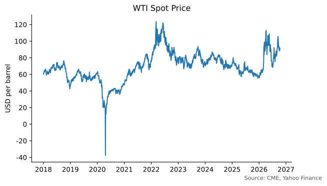
Negative Oil Prices
- April 2020: inventories rose and storage at Cushing, Oklahoma, the NYMEX delivery point, was filling up.
- On April 20, the day before expiration, traders long the May contract could not find buyers willing to take oil with no place to store it.
- The May contract, then the spot price, settled at about -\$38; the June contract settled at about $20.
- The spread of about $58 was the price of one month of storage at Cushing.
WTI Spot Price
Forwards vs. Futures
Valuing an Existing Forward Contract
- A forward contract is worth zero when it is first negotiated.
- Afterwards it may have a positive or negative value.
- Suppose that K is the delivery price and F is the forward price for a contract that would be negotiated today.
- Offsetting the old contract with a new one at F locks in a sure cash flow at T:
- The value of a long forward contract is (F - K) e^{-r T}.
- The value of a short forward contract is (K - F) e^{-r T}.
Example: Valuing an Existing Forward Position
- You entered into a short forward contract some time ago when the forward price was $200.
- Today the contract has 6 months until maturity and the current forward price is $190.
- The current risk-free rate is 5% per year with continuous compounding.
- If we buy a forward today, that would lock in a certain cash flow in six months of 200 - 190 = \$10.
- The present value today of this cash flow is 10 e^{-0.05 \times 6/12} = \$9.75 which is the value of the short forward contract.
Futures vs. Forward Prices
- Futures settle daily, so a futures position is worth zero after each settlement; forwards settle at maturity.
- If interest rates are deterministic, futures and forward prices are equal.
- Positive correlation between rates and the futures price: futures price above forward price, since gains arrive when rates are high.
- Negative correlation: the reverse, as for SOFR futures, whose price (100 - rate) falls when rates rise.
- For interest rate futures, traders adjust the observed futures rate to obtain the forward rate: a convexity adjustment.
Futures Prices vs.
Expected Spot Prices
Predicting Future Prices
- Futures prices are unbiased predictors of future spot prices only if investors require no risk premium.
- Let \mu be the rate at which investors discount a claim to one unit of the asset at T.
- \mu - r is the risk premium, from systematic risk or from hedgers paying speculators.
- Valuing one unit of the asset at T two ways, discounting \operatorname{E}(S_{T}) at \mu or a sure F at r: F e^{-r T} = \operatorname{E}(S_{T}) e^{-\mu T} \quad \Rightarrow \quad F = \operatorname{E}(S_{T}) e^{(r - \mu) T}
Futures Prices and the Risk Premium
| Risk Premium | Expected Return | Futures vs. Expected Price |
|---|---|---|
| Zero | \mu = r | F = \operatorname{E}(S_{T}) |
| Positive | \mu > r | F < \operatorname{E}(S_{T}) |
| Negative | \mu < r | F > \operatorname{E}(S_{T}) |
- Determining the risk premium of a commodity is not an easy task in practice.
The Evidence on Commodity Premiums
- Keynes (1930) and Hicks (1939): net short hedgers pay speculators, so \mu > r. Working (1953): hedgers are merchants trading the basis.
- Telser (1958): no upward drift in cotton and wheat futures.
- Cootner (1960): hedging is net short after the harvest and can be net long before, so the premium changes sign over the season.
- Dusak (1973): systematic risk and average returns near zero for wheat, corn, and soybean futures.
- Bessembinder (1992): hedgers’ net positions still predict returns. Gorton et al. (2013): inventories do, positions do not.
References
Bessembinder, Hendrik. 1992. “Systematic Risk, Hedging Pressure, and Risk Premiums in Futures Markets.” Review of Financial Studies 5 (4): 637–67.
Cootner, Paul H. 1960. “Returns to Speculators: Telser Versus Keynes.” Journal of Political Economy 68 (4): 396–404.
Dusak, Katherine. 1973. “Futures Trading and Investor Returns: An Investigation of Commodity Market Risk Premiums.” Journal of Political Economy 81 (6): 1387–406.
Gorton, Gary B., Fumio Hayashi, and K. Geert Rouwenhorst. 2013. “The Fundamentals of Commodity Futures Returns.” Review of Finance 17 (1): 35–105.
Hicks, John R. 1939. Value and Capital. Clarendon Press.
Keynes, John Maynard. 1930. A Treatise on Money. Macmillan.
Telser, Lester G. 1958. “Futures Trading and the Storage of Cotton and Wheat.” Journal of Political Economy 66 (3): 233–55.
Working, Holbrook. 1953. “Futures Trading and Hedging.” American Economic Review 43 (3): 314–43.