The Black-Scholes Model

Options, Futures and Derivative Securities

Lorenzo Naranjo

Spring 2026

Pricing Formulas

• Consider a non-dividend paying stock S that follows a GBM under the risk-neutral measure: dS = r S dt + \sigma S dB
• The price of European call and put options with strike price K and time-to-maturity T are given by: \begin{align*} C & = S \operatorname{Φ}(d_{1}) - K e^{-r T} \operatorname{Φ}(d_{2}) \\ P & = K e^{-r T} \operatorname{Φ}(-d_{2}) - S \operatorname{Φ}(-d_{1}) \end{align*} where \begin{align*} d_{1} & = \frac{\ln(S/K) + (r + \frac{1}{2} \sigma^{2}) T}{\sigma \sqrt{T}} \\ d_{2} & = d_{1} - \sigma \sqrt{T} \end{align*}

The Replicating Portfolio Approach

• Consider a derivative V written on a non-dividend paying stock S with maturity T that pays F(S) at maturity.
• The binomial model implies that the derivative can be replicated by buying (or selling) N_{S, t} units of the stock and N_{Z, t} units of a bond with face value K and maturity T, respectively.
• If we call V the value of such replicating portfolio, we have that at time t < T: V_{t} = N_{S, t} S_{t} + N_{Z, t} Z_{t}.
• In order to replicate the derivative, we want to make sure that the value of the portfolio at time t = T is equal to the payoff of the derivative, that is: V_{T} = H_{T}
• For example, for a European call option H_{T} = \max(S_{T} - K, 0).

The Replicating Portfolio is Self-Financing

• At time t+\Delta t, the value of the replicating portfolio is: V_{t + \Delta t} = N_{S, t} S_{t + \Delta t} + N_{Z, t} Z_{t + \Delta t}, which implies that: \Delta V_{t} = N_{S, t} \Delta S_{t} + N_{Z, t} \Delta Z_{t}.
• The new composition of the portfolio at time t+\Delta t is chosen such that: V_{t + \Delta t} = N_{S, t} S_{t + \Delta t} + N_{Z, t} Z_{t + \Delta t} = N_{S, t + \Delta t} S_{t + \Delta t} + N_{Z, t + \Delta t} Z_{t + \Delta t} which implies no matter what you do, you keep the value of the replicating portfolio unchanged, i.e., the portfolio is self-financing.

Replication in Continuous-Time

• As \Delta t \rightarrow 0, we have that: \begin{align*} dV & = N_{S} dS + N_{Z} dZ \\ & = N_{S} dS + N_{Z} (r Z dt) \\ & = N_{S} dS + (N_{Z} Z) r dt \\ \end{align*}
• And since V = N_{S} S + N_{Z} Z \Rightarrow N_{Z} Z = V - N_{S} S, we can conclude that: dV = r (V - N_{S} S) dt + N_{S} dS

Applying Ito’s Lemma

• We will assume for the moment that V is a smooth function of S and t, that is, V = V(S,t).
• Then, Ito’s Lemma implies that: \begin{align*} dV & = \frac{\partial V}{\partial S} dS + \frac{1}{2} \frac{\partial^{2} V}{\partial S^{2}} (dS)^{2} + \frac{\partial V}{\partial t} dt \\ & = \left(\frac{1}{2} \sigma^{2} S^{2} \frac{\partial^{2} V}{\partial S^{2}} + \frac{\partial V}{\partial t}\right) dt + \frac{\partial V}{\partial S} dS \end{align*}
• Therefore: \left(\frac{1}{2} \sigma^{2} S^{2} \frac{\partial^{2} V}{\partial S^{2}} + \frac{\partial V}{\partial t}\right) dt + \textcolor{blue}{\frac{\partial V}{\partial S} dS} = r (V - N_{S} S) dt + \textcolor{blue}{N_{S} dS}

The Delta of the Derivative

• First, the previous equation shows that replication works if and only if: N_{S} = \frac{\partial V}{\partial S}
• This is a fundamental relationship in derivatives pricing.
• It states that the number of shares needed to replicate the derivative is equal its sensitivity to the underlying asset.
• We call this quantity the delta (\Delta) of the derivative.
• Also, note that by choosing N_{S} equal to the delta of the derivative, it really does not matter what drift we have for the stock.
• We will use this fact in a moment to define the risk-neutral probabilities in continuous-time.

The Fundamental Partial Differential Equation (PDE)

• Second, it must be the case that: \frac{1}{2} \sigma^{2} S^{2} \frac{\partial^{2} V}{\partial S^{2}} + \frac{\partial V}{\partial t} = r \left(V - S \frac{\partial V}{\partial S}\right)
• Therefore: \frac{\partial V}{\partial t} + \frac{1}{2} \sigma^{2} S^{2} \frac{\partial^{2} V}{\partial S^{2}} + r S \frac{\partial V}{\partial S} - r V = 0 subject to V_{T} = H_{T}.
• This is the celebrated Black-Scholes partial differential equation (PDE) which allowed the authors to compute their influential formula in 1973!
• Solving PDEs, in general, is very hard so we will resort to a different approach to price European call and put options.

The Risk-Neutral Pricing Approach

• The replicating approach is insensitive to the drift of the stock.
• As a matter of fact, the drift might even change based on whose thinking about the asset.
• Since the previous reasoning is silent about the drift and the type of investor pricing the asset, we can assume in our reasoning that all investors are .
• Even if this is not true in real markets, such assumption would not affect of the replicating-portfolio argument.

A Risk-Neutral World

• In a world populated by risk-neutral investors, the price today of any non-dividend paying asset is equal to the expected payoff at maturity discounted at the risk-free rate, that is: X = e^{-rT} \operatorname{E}^{*}(X_{T})
• Therefore, the drift of a non-dividend paying stock is the risk-free rate: dS = r S dt + \sigma S dB^{*}
• The same is true for all derivatives written on the stock: dV = \underbrace{\left(r S \frac{\partial V}{\partial S} + \frac{1}{2} \sigma^{2} S^{2} \frac{\partial^{2} V}{\partial S^{2}} + \frac{\partial V}{\partial t}\right)}_{=rV} dt + \left(\sigma S \frac{\partial V}{\partial S}\right) dB^{*}
• We recover the same equation as before!

Pricing a European Call Option

• Consider a European call option written on a non-dividend paying stock with maturity T and strike price K.
• The price of the call should then be: \begin{align*} C & = e^{-r T} \operatorname{E}\left((S_{T} - K) 1\kern-0.25em\text{l}_{\{S_{T} > K\}} \right) \\ & = e^{-r T} \operatorname{E}\left(S_{T} 1\kern-0.25em\text{l}_{\{S_{T} > K\}} \right) - e^{-r T} \operatorname{E}\left(K 1\kern-0.25em\text{l}_{\{S_{T} > K\}} \right) \\ & = S \operatorname{Φ}(d_{1}) - K e^{-r T} \operatorname{Φ}(d_{2}) \end{align*} where \begin{align*} d_{1} & = \frac{\ln(S/K) + (r + \frac{1}{2} \sigma^{2}) T}{\sigma \sqrt{T}} \\ d_{2} & = d_{1} - \sigma \sqrt{T} \end{align*}

Call Premium vs. Spot Price

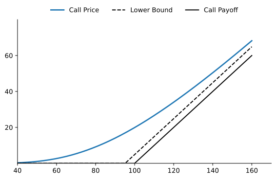
The figure plots the Black-Scholes call premium C(S) if r=0.05, \sigma=0.45, T=1 and K=100. It also shows the call option payoff given by \max(S - K, 0) and the lower bound for a European call given by \max(S - K e^{-r T}, 0).

Reconciling Both Pricing Approaches

• It is tedious but straightforward to prove that: \begin{equation} N_{S} = \frac{\partial C}{\partial S} = \operatorname{Φ}(d_{1}) \end{equation} \tag{1}
• Also, we have that for a European call option: C = N_{S} S + N_{Z} Z = S \operatorname{Φ}(d_{1}) - K e^{-r T} \operatorname{Φ}(d_{2}) which because of implies that: N_{Z} = -\operatorname{Φ}(d_{2})

Call Delta

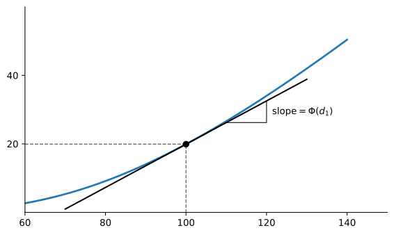
The figure plots the Black-Scholes call premium C(S) where r = 0.05, \sigma = 0.45, T = 1 and K = 100, and shows the tangent line at S = 100 whose slope coefficient is the delta of the call given by \operatorname{Φ}(d_{1}).

Hedging the Call

• Our analysis so far implies that to replicate a European call option, we need to go \operatorname{Φ}(d_{1}) shares of stock and \operatorname{Φ}(d_{2}) risk-free bonds with face value K and maturity T.
• The call is therefore a levered position in the underlying asset whose delta is given by \operatorname{Φ}(d_{1}).
  • Since 0<\operatorname{Φ}(d_{1})<1, the delta of the call for a non-dividend paying asset is bounded between 0 and 1.
• As we saw in the previous slide, for a given spot price, the delta of the call represents the slope coefficient of the tangency line at that point.

Pricing a European Put Option

• Consider now a European put option with the same characteristics as the previous call.
• According to put-call parity, it must be the case that: ` C - P = S - K e^{-r T}
• Hence, \begin{align*} P & = C - (S - K e^{-rT}) \\ & = S \operatorname{Φ}(d_{1}) - K e^{-r T} \operatorname{Φ}(d_{2}) - (S - K e^{-rT}) \\ & = K e^{-r T} (1 - \operatorname{Φ}(d_{2})) - S (1 - \operatorname{Φ}(d_{1})) \\ & = K e^{-r T} \operatorname{Φ}(-d_{2}) - S \operatorname{Φ}(-d_{1}) \end{align*}

Put Premium vs. Spot Price

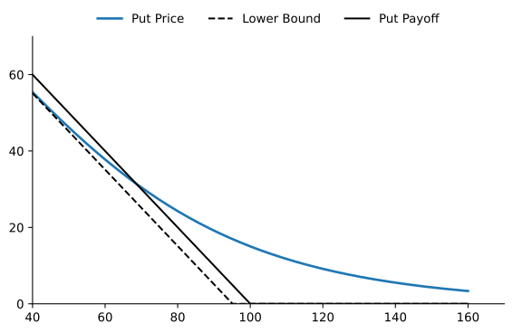
The figure plots the Black-Scholes put premium P(S) if r = 0.05, \sigma = 0.45, T = 1 and K = 100. It also shows the put option payoff given by \max(K - S, 0) and the lower bound for a European put given by \max(K e^{-r T} - S, 0).

Put Delta

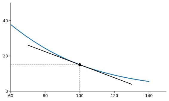
The figure plots the Black-Scholes put premium P(S) where r = 0.05, \sigma = 0.45, T = 1 and K = 100, and shows the tangent line at S = 100 whose slope coefficient is the delta of the put given by -\operatorname{Φ}(-d_{1}) = \operatorname{Φ}(d_{1}) - 1.

Hedging the Put

• We can use put-call parity to compute N_{S} for the put: N_{S} = \frac{\partial P}{\partial S} = \frac{\partial (C - S + K e^{-rT})}{\partial S} = \operatorname{Φ}(d_{1}) - 1 = -\operatorname{Φ}(-d_{1}) < 0
• The fact that we also have P = N_{S} S + N_{Z} Z also implies that: N_{Z} = \operatorname{Φ}(-d_{2}) > 0
• Therefore, to replicate a European put option, we need to go \operatorname{Φ}(-d_{1}) shares of stock and \operatorname{Φ}(-d_{2}) risk-free bonds with face value K and maturity T.

Finishing In-The-Money

• Remember that we showed that: \operatorname{P}(S_{T} > K) = \operatorname{E}\left(1\kern-0.25em\text{l}_{\{S_{T} > K\}}\right) = \operatorname{Φ}(d_{2}) which also implies that: \operatorname{P}(S_{T} < K) = 1 - \operatorname{P}(S_{T} > K) = 1 - \operatorname{Φ}(d_{2}) = \operatorname{Φ}(-d_{2})
• Therefore, the risk-neutral probability that the call will expire in-the-money is equal to \operatorname{Φ}(d_{2}) whereas the risk-neutral probability that the put finishes in-the-money is given by \operatorname{Φ}(-d_{2}).

Example 1 Consider a non-dividend paying stock that currently trades for $100. The risk-free rate is 4% per year, continuously compounded and constant for all maturities. The instantaneous volatility of returns is 25% per year. Consider at-the-money call and put options written on the stock with maturity 9 months. Then, \begin{align*} d_{1} & = \frac{\ln(100/100) + (0.04 + 0.5(0.25)^{2})(0.75)}{0.25\sqrt{0.75}} = 0.2468 \\ d_{2} & = 0.2468 - 0.25\sqrt{0.75} = 0.0303 \end{align*} Therefore, \operatorname{Φ}(d_{1}) = 0.5975 and \operatorname{Φ}(d_{2}) = 0.5121, which implies that: \begin{align*} C & = 100(0.5975) - 100e^{-0.04(0.75)}(0.5121) = \$10.05 \\ P & = 100e^{-0.04(0.75)}(1 - 0.5121) - 100(1 - 0.5975) = \$7.10 \end{align*}

The Impact of Volatility

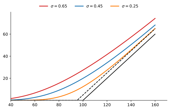
The figure shows the Black-Scholes call premium for different levels of volatility where r = 0.05, T = 1 and K = 100. The dashed line represents the lower bound for the European call and the solid black line is the call payoff at maturity.

Option Premium vs. Volatility

• One of the most important determinants of option prices in the Black-Scholes model is volatility.
• We can show that for European call and put options: \begin{equation} \frac{\partial C}{\partial \sigma} = \frac{\partial P}{\partial \sigma} = S \mathop{\Phi^{'}}(d_{1}) \sqrt{T} > 0 \end{equation} \tag{2}
• Hence, both European call and put options increase in value as volatility increases.
• Moreover, this also implies that there is a one-on-one relationship between option value and volatility, i.e., we can use volatility to quote prices and vice-versa.
• The volatility that matches the observed price of an option is called the implied volatility.

Example 2 Consider a non-dividend paying stock that currently trades for $100. The risk-free rate is 5% per year, continuously compounded and constant for all maturities. An ATM European call option written on the stock with maturity 12 months trades for $16. We can check that \sigma=34.66\% prices the call correctly: \begin{align*} d_{1} & = \frac{\ln(100/100) + (0.05 + 0.5(0.3466)^{2})(1)}{0.3466\sqrt{1}} = 0.3176 \\ d_{2} & = 0.3358 - 0.3466\sqrt{1} = -0.0290 \\ \end{align*} Therefore, \operatorname{Φ}(d_{1}) = 0.6246 and \operatorname{Φ}(d_{2}) = 0.4884, which implies that C = 100(0.6246) - 100e^{-0.05(1)}(0.4884) = \$16.00

How Can We Compute the Implied Volatility?

• Unfortunately, it is not possible to solve analytically for the implied volatility.
• For a call option, for example, it involves solving numerically for \sigma: C = C(\sigma_{\mathit{imp}})
• Alternatively, we could tabulate the price of a call option for different values of \sigma (using the same parameters as the previous example):

\sigma	0.05	0.10	0.15	0.20	0.25	0.30	0.35	0.40
C	5.28	6.80	8.59	10.45	12.34	14.23	16.13	18.02

• We can see that \sigma=35\% gives a price of \$16.13 for the call, which is quite close to the true implied volatility of 34.66%.

Implied Volatility for a Call Option

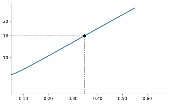
The figure shows the Black-Scholes call premium C(\sigma) as a function of \sigma where S=100, r = 0.05, T = 1 and K = 100. We can see that for C = \$16 the corresponding volatility is approximately 35%.