Plotting the SPX Implied Volatility Surface with WRDS

How to pull SPX options data from OptionMetrics via WRDS and build an average implied volatility surface in Python.

The implied volatility surface is one of the most useful diagnostic tools in options markets. It shows, at a glance, how the market prices risk across strikes and maturities — and how that pricing deviates from the flat surface Black-Scholes would predict. The steep skew on the left (low moneyness, high IV) reflects the market’s persistent demand for downside protection on the S&P 500.

This post shows how to pull SPX options data from OptionMetrics via WRDS, filter to OTM puts and calls, and build an average surface across a full year of trading days.

Pulling data from WRDS

OptionMetrics on WRDS stores options data in annual tables. We query two years, filter to SPX (secid 108105), and grab the underlying close price from the security price table.

import wrds
import numpy as np
import pandas as pd

db = wrds.Connection()

opts = db.raw_sql("""
    SELECT date, exdate, cp_flag, strike_price, impl_volatility
    FROM optionm_all.opprcd2024
    WHERE secid = 108105
      AND date >= '2024-08-01'
    UNION ALL
    SELECT date, exdate, cp_flag, strike_price, impl_volatility
    FROM optionm_all.opprcd2025
    WHERE secid = 108105
      AND date <= '2025-08-31'
""", date_cols=["date", "exdate"])

spx = db.raw_sql("""
    SELECT date, close
    FROM optionm_all.secprd2024
    WHERE secid = 108105
      AND date >= '2024-08-01'
    UNION ALL
    SELECT date, close
    FROM optionm_all.secprd2025
    WHERE secid = 108105
      AND date <= '2025-08-31'
""", date_cols=["date"])

db.close()

Loading library list...
Done

Filtering to OTM options

We compute moneyness as \(K/S\) and time to expiry in years, then keep only OTM puts (moneyness < 1) and OTM calls (moneyness ≥ 1). Note that OptionMetrics stores strike_price scaled by 1000, so we divide before computing moneyness. Using OTM options avoids the bid-ask noise that plagues deep in-the-money contracts and gives us the cleanest read on the skew.

opts = opts.merge(spx, on="date").copy()
opts.loc[:, "moneyness"] = opts["strike_price"] / 1000 / opts["close"]
opts.loc[:, "T_years"] = (opts["exdate"] - opts["date"]).dt.days / 365

tmp = (
    opts[["date", "moneyness", "T_years", "impl_volatility", "cp_flag"]]
    .dropna()
    .query("impl_volatility < 0.8 and T_years > 0.08 and T_years < 1.5 and moneyness >= 0.7 and moneyness <= 1.3")
)
tmp = tmp[
    ((tmp["cp_flag"] == "P") & (tmp["moneyness"] < 1)) |
    ((tmp["cp_flag"] == "C") & (tmp["moneyness"] >= 1))
]

The IV cap of 0.8 is intentionally generous — the left tail of the SPX skew can exceed 60% for deep OTM puts, especially during stress periods, and cutting too aggressively there is exactly where you lose the interesting part of the surface.

Building the average surface

For each trading day, we interpolate the available (moneyness, maturity, IV) triples onto a common 80×80 grid using linear interpolation. We then average across days, discarding grid points that lack data on at least 5% of trading days.

from scipy.interpolate import griddata
from scipy.ndimage import gaussian_filter
import warnings

mg = np.linspace(0.7, 1.3, 80)
Tg = np.linspace(0.08, 1.5, 80)
MM, TT = np.meshgrid(mg, Tg)

surfaces = []
for date, grp in tmp.groupby("date"):
    m  = grp["moneyness"].to_numpy()
    T  = grp["T_years"].to_numpy()
    iv = grp["impl_volatility"].to_numpy()
    if len(m) < 10:
        continue
    ZZ = griddata(np.c_[m, T], iv, (MM, TT), method="linear")
    surfaces.append(ZZ)

stack    = np.stack(surfaces)
coverage = np.sum(~np.isnan(stack), axis=0)
with warnings.catch_warnings():
    warnings.simplefilter("ignore", RuntimeWarning)
    ZZ = np.nanmean(stack, axis=0)
ZZ[coverage < len(surfaces) * 0.05] = np.nan

The gaussian smoothing below is a weighted blur that respects missing values — it avoids smearing NaNs into valid regions at the surface boundary.

valid    = ~np.isnan(ZZ)
ZZ_filled = np.where(valid, ZZ, 0.0)
w        = gaussian_filter(valid.astype(float), sigma=2.5)
w_safe   = np.where(w > 0, w, 1.0)
ZZ       = np.where(w > 0, gaussian_filter(ZZ_filled, sigma=2.5) / w_safe, np.nan)

The surface

import matplotlib.pyplot as plt

fig = plt.figure(figsize=(7, 5))
ax  = fig.add_subplot(111, projection="3d")
ax.plot_surface(TT, MM, ZZ, cmap="jet", linewidth=0.3, edgecolor="white",
                alpha=0.95, rstride=1, cstride=1)
ax.set_xlabel("Maturity", labelpad=8)
ax.set_ylabel("Moneyness (K/S)", labelpad=8)
ax.set_zlabel("Implied Volatility", labelpad=8)
ax.invert_yaxis()
ax.view_init(elev=25, azim=210)
plt.tight_layout()
plt.show()

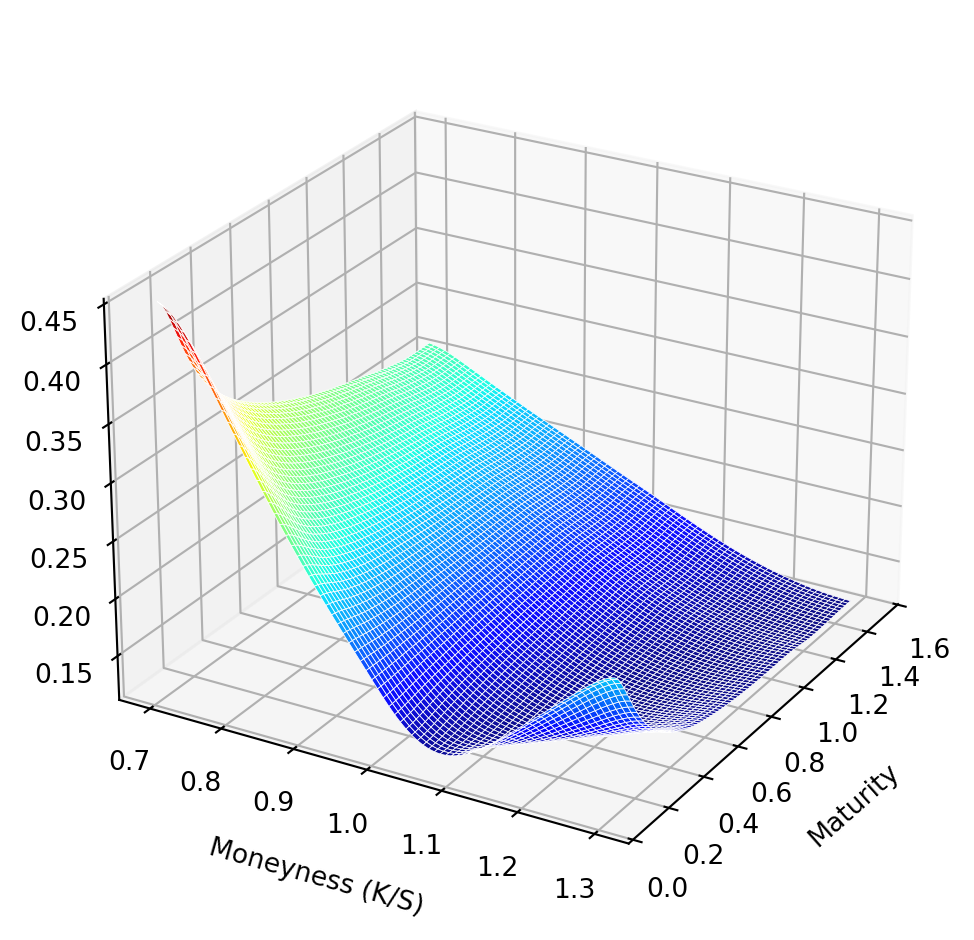
Figure 1: Average implied volatility surface for SPX options, using OTM puts (K/S < 1) and OTM calls (K/S ≥ 1) interpolated to a common moneyness–maturity grid and averaged over 251 trading days (August 2024 – August 2025).

The volatility skew is the dominant feature — implied volatility rises sharply as moneyness falls below 1, reflecting the premium the market charges for put protection. The term structure is flatter, with short-dated ATM volatility running slightly above longer-dated levels, consistent with a market pricing near-term uncertainty at a modest premium to longer-run risk.